
This content originally appeared on Level Up Coding - Medium and was authored by Aaron Li
“One step behind” is a series of blogs I’ll be writing after I learn a new ML concept.
My current situation
- Just finished the Fourth lesson of Fast AI (including the previous ones)
Note: Contents of this article will come from the third lesson of FAST AI
What you’ll need to know for this article
- High school math
- Python knowledge
- Mean squared error
- PyTorch (Not much actually, will explain the codes along with the article)
- The behavior of quadratic function (IE. how the coefficient of x² affect the concavity of the function)
Is this article for you?
This article is the second one in the series “One step behind”. Reading the first article would help to understand this if you have minimum prior knowledge about machine learning. In this article, I’ll be discussing how a machine learns using high school math. If you’re interested in the scenes behind machine learning, then this article might be for you. Prior experience in training ML models would help a lot in understanding this article even if you just read other’s code and ran it with no clue.
Why it’s intimidating to learn ML and why it’s not supposed to be
The field of machine learning is no doubt interesting; however the amount of fancy vocabulary in ML is quite intimidating. In reality, a lot of the jargon is actually just high school math hiding behind fancy words.
This was a problem for me when I was initially starting to learn ML. Simple concepts wrapped by jargon would usually get me stuck as I would still need to search and try to understand them. Among the several ways I used to learn ML, the most effective so far was FAST AI’s online course. It uses the top-down approach but while doing so, they won’t intimidate you with fancy words, as they abstractly tell you what these results to without you having to worry about falling behind the lesson.
Contents of this article
In this article, we will see how a machine learns with concepts as simple as for loops.
Tips before starting
Your learning experience will be better if you follow along. Here is the colab notebook of the code mentioned below.
https://colab.research.google.com/drive/1fr-hhP2tFpn6ENBBqk8AafyNgBsB86Ub?usp=sharing
Note: Running the first cell of the notebook would take a while. Enter the authorization code generated for you to mount it your drive.
Lets get started
Suppose we arrange for some automatic means of testing the effectiveness of any current weight assignment in terms of actual performance and provide a mechanism for altering the weight assignment so as to maximize the performance. We need not go into the details of such a procedure to see that it could be made entirely automatic and to see that a machine so programmed would “learn” from its experience.
-Arthur Samuel
The quote above by Arthur Samuel tells us the essence of machine learning. Our goal today is to understand this quote above.

The image is a graphical representation of the quote.
Problem: We want to find a function that will give us the speed of the roller coaster at a point in time.
Given: We are given data captured by a rider with a speedometer.

Above is time vs speed graph, a representation of the data the rider captured at several point of his ride.
Sample interpretation: At 2.6 seconds, the roller coaster was moving at 25 meters per second.
Looking at it, we can deduce that it can be modeled with a quadratic function. That said, we want to create a quadratic function that closely resembles the one above. (Creating a quadratic function doesn’t mean we draw it, but rather get the actual numerical values of it)
Quadratic functions in python
First, we want to make a quadratic function in python. This is a good time to recall high school lessons, more specifically functions. As we know, a quadratic function looks is structured like this: f(x) = ax² + bx + c. Compare it to the python function below.
def f(t, params):
a,b,c = params
return a*(t**2) + (b*t) + c
Perhaps you are already starting to see the resemblance between them. And yes, they are essentially the same thing. The only difference is that x is replaced with t which doesn’t really matter because they are just variables. We use t here because its much more logical to use t to represent time.
Knowing how correct or wrong we are
def mse(preds, targets):
return ((preds-targets)**2).mean().sqrt()
To determine how close we are to the correct answer, we’ll be using the mean squared error (MSE). The function above will take in the output of the quadratic function above and compare it with the actual value the rider acquired from the speedometer.
1st step in Arthur Samuel’s description: Initialize
params = torch.randn(3).requires_grad_()
For an easier understanding on how the code above works, I’ll be breaking it down.
torch.randn(3) — returns 3 random numbers, which will become our a,b,c (For reference: f(x) = ax² + bx + c)
requires_grad() — will allow PyTorch(the library we are using) to calculate gradient (you’ll understand why later)
Okay, so great! We now finished the first step. We now have a random quadratic function. It might not fit the data given very well but at least we got something to work on already.
2nd step: Predict
preds = f(time, params)
time here is a list of numbers .
Fitting the value of time in the quadratic function, the output of f() is the prediction.
Note: preds here is Rank 1 tensor (one-dimensional array) with several values in it.
Up to this point, you might start realizing that a prediction model is a quite similar to a function. Well, actually it is just a function. You give it a value of x, which in this case is the time, then it will give you the corresponding y-value of the x. Modeling, in this sense, is just finding the correct parameters so that this function will be able to have a correct y-value/prediction.
The image below shows us the results of our function(red dots) in comparison to the actual results(blue dots)
Note: There might be some differences as the functions are randomly initiated.

3rd step: Calculating Loss
Yes, we know that our predictions are wrong, but do we know how wrong they are? Here comes the mean squared error we defined earlier.
def mse(preds, targets):
return ((preds-targets)**2).mean().sqrt()
Calling it
loss = mse(preds, speed)
Our goal here is to minimize the loss. As our function starts to fit the data more, the difference between them will also start to decrease, thus the loss will also start to decrease as we get more accurate.
4th step: Calculating the gradient
Here comes another high school mathematics concept. Gradient may seem a little bit abstract to you since, you probably just remember that:
f(x) = x²
f’(x) = 2x
Gradient in another word is just the slope of a function(rise over run). In a linear function, you can get it easily as the slope is always constant, but in a quadratic function the slopes are often changing. This is the reason why we have variables in the derivative/gradient of x². As the values of x changes, the slope also changes.
With that said, the next step is to calculate the gradients of the parameters.
loss.backward()
params.grad
Gradient of the parameters is confusing to think of. So in simple terms, this block of code above will tell you how the change in parameters affect the change in loss.
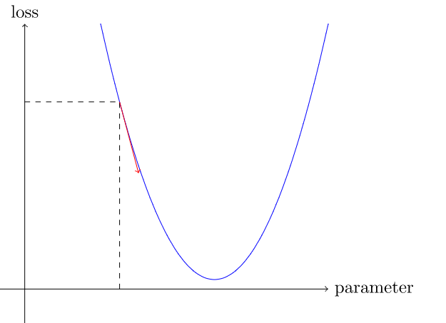
With this we now know which direction we could change the parameters (x-axis) in order to reduce the loss (y-axis)
Note: The graph above is not the same as the one with red and blue dots. This one represents the relationship between our loss and parameters, while the one above gives a comparison between the actual data points and the predicted data points.
5th step: Changing the weights
Looking at the title of this section, you might start wondering why the word “weights” just suddenly appeared out nowhere. Its a great time to tell you that weights are the parameters of the model. These are the values that you put in the model’s parameter.
For example:
f(x) = ax² + bx + c
Here, a, b, and c are the parameters of the model.
f(x) = 2x² + 3x + 4
2, 3, and 4 are the weights of the model.
Hope that clarifies weights and parameters.
Below is the code to update the weights:
lr = 1e-5
params.data -= lr * params.grad.data
params.grad = None
Lets take a look at it one by one.
lr = 1e-5
lr refers the learning rate of the model, which in this case is 1 raised to -5. From the gradients we calculated earlier, we know which direction and how steep the direction is.

The larger the learning rate the bigger step we take in the x-axis, this will make it learn faster but it may also have the opposite effect as it will take too big of a step that will make it miss the point with the smallest loss value. On the other hand a small learning rate will make it more accurate as it will take more steps meaning that there is a lesser chance that it will miss the minimum loss value; however this will take a longer time to perform.
You can try different learning rates after learning how the whole thing works, but for now we’ll just use 1 raised to -5.
params.data -= lr * params.grad.data
Having the learning rate and the gradient we can start changing the values of the parameters to go one step closer to our goal of having a lower value of loss. In order to not affect our gradient while tweaking the params is to add .data. Because we declared earlier [.requires_grad()] that we want PyTorch to remember the operations done on the parameters for knowing the gradient, tweaking this params is also going to be included in the recording of operations. We wouldn’t want this because the only time we want our gradient is during the predicting stage.
params.grad = None
This step just deletes the gradient to give space for the next gradient in the next prediction.
Lets go back to Step 2: Predict and Step 3: Calculate Loss
Now we have changed the weights of the model, we can check if the loss has lowered.
Run the codes in step 2 and 3 again:
Predict
preds = f(time, params)
Find loss
loss = mse(preds, speed)
loss
In my case, my loss has lowered from 143.6154 to 143.3416
Lets compile these so that we can run them a lot of times using a for loop
def learn():
preds = f(time, params)
loss = mse(preds, speed)
loss.backward()
params.data -= lr * params.grad.data
params.grad = None
print(“loss: “ + loss[0])
Running it in a for loop
for i in range(10):
learn()
Below is the results of my loss:
tensor(142.2465, grad_fn=<SqrtBackward>)
tensor(141.9728, grad_fn=<SqrtBackward>)
tensor(141.6992, grad_fn=<SqrtBackward>)
tensor(141.4256, grad_fn=<SqrtBackward>)
tensor(141.1520, grad_fn=<SqrtBackward>)
tensor(140.8785, grad_fn=<SqrtBackward>)
tensor(140.6050, grad_fn=<SqrtBackward>)
tensor(140.3315, grad_fn=<SqrtBackward>)
tensor(140.0581, grad_fn=<SqrtBackward>)
tensor(139.7847, grad_fn=<SqrtBackward>)
Step 7: Stop
After nearly a thousand loops:
tensor(25.1210, grad_fn=<SqrtBackward>)
My loss value was around 25 after approximately a thousand loops. It just maintained at this value for a while so I just decided to stop.
Conclusion
Congratulations you created a machine learning model! Thank you for reaching the end of this article. It’s pretty amazing how simple mathematical concepts can generate magic-like results through the use of computers.
Machine Learning explained with high-school math was originally published in Level Up Coding on Medium, where people are continuing the conversation by highlighting and responding to this story.
This content originally appeared on Level Up Coding - Medium and was authored by Aaron Li
Aaron Li | Sciencx (2021-03-29T15:01:53+00:00) Machine Learning explained with high-school math. Retrieved from https://www.scien.cx/2021/03/29/machine-learning-explained-with-high-school-math/
Please log in to upload a file.
There are no updates yet.
Click the Upload button above to add an update.