
This content originally appeared on DEV Community and was authored by Rafael Rocha
Description
This post presents a simple regression problem through Polynomial Curve Fitting analysis. Besides, will explain some key concepts of machine learning, as generalization, overfitting, and model selection. The Pattern Recognition and Machine Learning book of Christopher M. Bishop inspires the post.
Data generation
Both training and validation sets are synthetically generated. The input variable X is generated by spaced uniformly random values in range [0, 1]. The output (or target data) variable y is generated from the generating function sin(2πx) added of random noise. The figure in the cover presents the curves of the target data (training set) and the generating function of N = 10 training examples.
Polynomial features
First, the input variable X (that represents one single feature) will be transformed to polynomial features (X_poly), according to the below function:
def poly_features(x, M):

  N = len(x)

  x_poly = np.zeros([N, M+1], dtype=np.float64)
  for i in range(N):
    for j in range(M+1):
      x_poly[i, j] = np.power(x[i], j)

  return x_poly
Thus, the column vector X of size N x 1 will result in a N x M + 1 matrix, where M is the order of the polynomial. For example, using M = 2 and x = 0.3077 results in three features as follows:
![]()
The figure below presents the polynomial features of three examples of the training set.

Training
The next step aims to train the model (with training data), that is, find the coefficients W that multiplied by polynomial features allow us to make predictions y_pred. There are some optimization algorithms, like gradient descent, that minimize the cost function, in this case, the error between the real value y and the predicted value y_pred. Here is used the normal equation to obtain W, as given by the equation (normal) below:
![]()
Where X is the polynomial features matrix of size N x M+1, y is the output variable of size N x 1, and W is the coefficients of size M+1 x 1. The coefficients obtained through normal equation are given by the function below:
def normal_equation(x, y):

    # Normal equation: w = ((x'*x)^-1) *x'*y

    xT = x.T
    w = np.dot(np.dot(np.linalg.pinv(np.dot(xT, x)), xT), y)

    return w
Measuring the error
With the coefficients W in hand, it is necessary to measure the error between the real value (output variable y) and the predicted value y_pred. It is used the Root-Mean Square Error (RMSE) obtained through the Sum-of-Squares Error (SSE) to evaluate the performance of the training model. The equations below obtain the errors:

![]()
Where N is the number of examples. The functions below calculate these errors:
def error(y, y_pred):

    N = len(y)

    # Sum-of-squares error
    sse = np.sum(np.power(y_pred-y, 2))/2

    # Root mean squere error
    rmse = np.sqrt(2*sse/N)

    return sse, rmse
Validation
The next step is to evaluate the validation set, which is data that was not in the model training. Here it is verified whether the model fits the validation set. Most steps are the same as training, how to get the polynomial features, make predictions and measure the error.
Polynomial order analysis
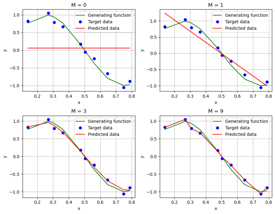
The figure below shows the four (M = 0, 1, 3, 9) different orders of the polynomial. The green curve represents the generating function, blue dots presents the target data (training data, X and y), and the red curve shows the predicted data (y_pred). The worst predictions are presented by M = 0, followed by M = 1. M = 3 and M = 9 are the ones who achieve the best prediction, that is, they are the models that best fit the training set.
Error analysis
Analyzing the RMSE (in the figure below), there is a tendency for the error to decrease in both training and validation between M = 0 and M = 3. But for M = 9, one notices a much bigger error in the validation set, that is, as the order of the polynomial grows it becomes more difficult for the model to predict examples outside the training set. In short, the model lacks the generalization ability. The behavior of M = 9 can be called overfitting.

The order of polynomial helps in selection model, which the choice is M = 3, as it is the model that has the smallest validation error.
One of the possible ways to prevent overfitting is to add more examples, in this case generating training and validation sets with N = 50, we obtain the RMSE by order of the polynomial as shown in the figure below:

Thus, when more examples are added, it is possible to prevent overfitting of the M = 9 model.
The complete code is available on Github and Colab. Follow the blog if the post it is helpful for you.
Follow me on Linkedin and Github.
This content originally appeared on DEV Community and was authored by Rafael Rocha
Rafael Rocha | Sciencx (2022-04-30T01:37:19+00:00) Curve Fitting: An explain of key concepts of machine learning. Retrieved from https://www.scien.cx/2022/04/30/curve-fitting-an-explain-of-key-concepts-of-machine-learning/
Please log in to upload a file.
There are no updates yet.
Click the Upload button above to add an update.