
This content originally appeared on Level Up Coding - Medium and was authored by MicroBioscopicData
Vectors are fundamental building blocks of various machine learning algorithms
Vectors are fundamental building blocks of linear algebra and play a crucial role in various machine learning algorithms. This comprehensive tutorial aims to equip you with a thorough understanding of vectors, covering their definition, function, interpretation, and implementation in Python. You will gain proficiency in essential vector operations such as algebra and dot products. Understanding the algebraic and geometric properties of vectors is essential for performing various operations in data analysis and machine learning, such as dimensionality reduction, clustering, and classification.
Table of contents:
· Algebraic and geometric view of vectors
· Vector Magnitude and Unit Vectors
· Vector addition and subtraction
· Vector-Scalar Multiplication
· Vector-vector multiplication (dot product)
Algebraic and geometric view of vectors
Linear algebra concepts can be effectively expressed and visualized through both algebraic and geometric representations, offering a powerful duality in understanding. This is because certain concepts are more intuitively grasped through algebraic representations (storing sales data over time), while others are better interpreted using geometric terms (geometric interpretation of a vector is useful in physics and engineering) [1]. By leveraging this dual approach, one can develop a more comprehensive understanding of linear algebra concepts and their practical applications.
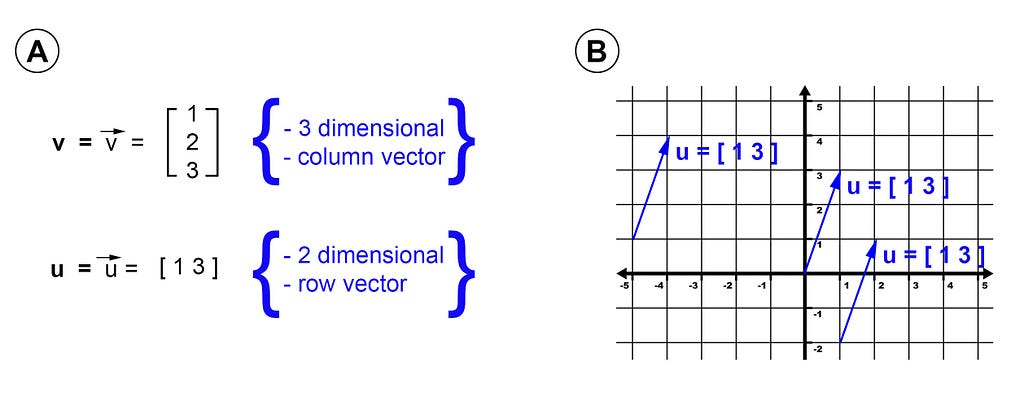
A vector can be represented algebraically as an ordered list of components, typically numeric values, where the sequence of these components has a specific meaning [2]. Each component in a vector is referred to as an element, and the total number of elements within a vector is known as its dimensionality (Figure 1A). Vectors can be represented in two orientations — column orientation (standing up tall) or row orientation (laying flat and wide). The standard notation for representing vectors is using a lowercase, bold Latin letter (sometimes augmented with an arrow symbol above the letter).
When looking at the geometric interpretation of vectors, we can visualize a vector as a straight line with a defined length and direction in space. The length of the vector represents its magnitude (see below), while the direction is indicated by the orientation of the vector in relation to a reference point or axis. While vectors are typically drawn starting at the origin of a graph (this is called the standard position), they can be positioned anywhere in space without affecting their properties. In fact, the direction and magnitude of a vector remain the same regardless of its starting point, as long as its endpoint remains the same (Figure 1B). The starting point of a vector is referred to as the tail, while the endpoint, typically drawn with an arrowhead, is referred to as the head of the vector. Visualizing vectors in this way allows us to better understand and manipulate them, providing a useful tool for analyzing the relationships between features in a dataset, making them an essential concept in machine learning and data science.
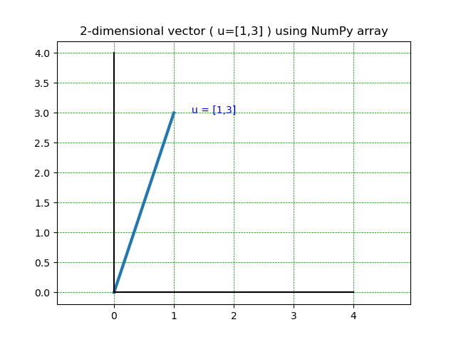
In Python, vectors can be expressed through different data types. While using a list type may seem like a straightforward approach to representing a vector, it may not be suitable for certain applications that require linear algebra operations [1]. Hence, creating vectors as NumPy arrays is often preferred as they allow for more efficient and effective operations (Figure 2).
# Create the vector as NumPy array
u = np.array([1,3])

# plot the vector
plt.plot([0,u[0]],[0,u[1]], lw=3)
plt.axis('equal')
plt.plot([0, 4],[0, 0],'k-')
plt.plot([0, 0],[0, 4],'k-')
plt.grid(color = 'green', linestyle = '--', linewidth = 0.5)
plt.xticks(np.arange(0, 5, 1))
plt.title("2-dimensional vector ( u=[1,3] ) using NumPy array")

# Annotate the vector
plt.annotate("u = [1,3]", xy=(1+0.3,3), color ="blue")
Output:
Vector Magnitude and the Unit Vectors
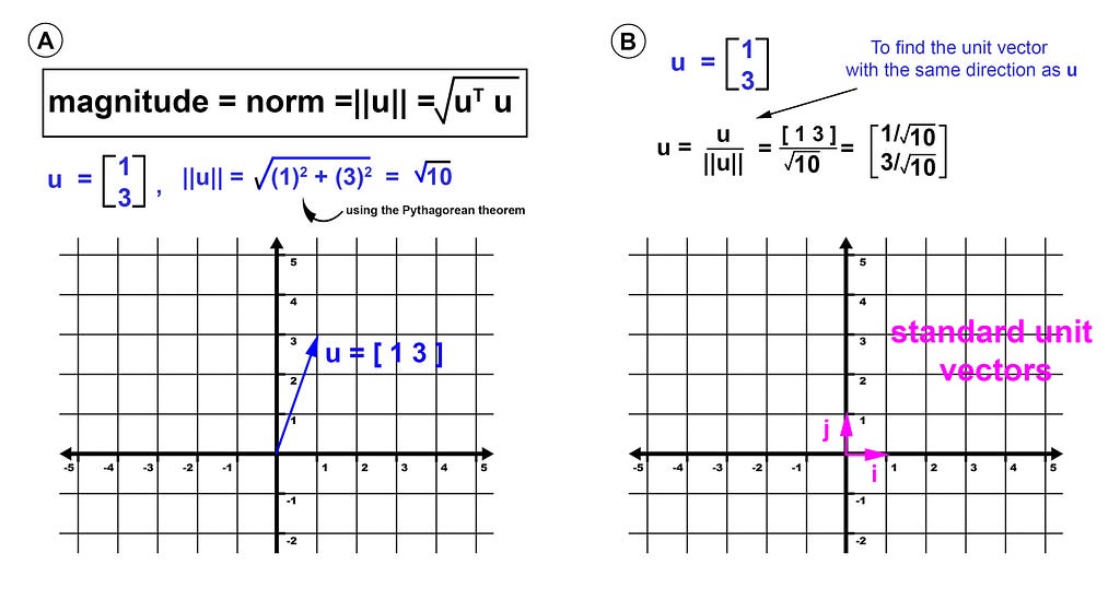
The magnitude of a vector, also known as its geometric length or norm, is determined by the distance from its tail to head. It is calculated using the standard Euclidean distance formula (Figure 3A). In mathematics, the Euclidean distance between two points in Euclidean space is the length of a line segment between the two points. It can be calculated from the Cartesian coordinates of the points using the Pythagorean theorem, and is sometimes referred to as the Pythagorean distance [3]. Vector magnitude is denoted using double vertical bars around the vector, as in ∥ v ∥ (Figure 3A).
There are some applications where we want a vector that has a geometric length of one, which is called a unit vector (sometimes referred to as a direction vector). Example applications include orthogonal matrices, rotation matrices, eigenvectors, and singular vectors [2]. The unit vectors are denoted by the “cap” symbol ^ and are defined as magnitude = ∥ v ∥ = 1. For example, vector u = (1, 3) is not a unit vector, because its magnitude is not equal to 1 (i.e., ||v|| = √(12+32) ≠ 1) (Figure 3A). Any vector can become a unit vector when we divide it by the magnitude of the same given vector (Figure 3B). i, and j, are special unit vectors (also called standard unit vectors) that are parallel to the coordinate axes in the directions of the x-axis and y-axis, respectively in a 2-dimensional plane. i.e.,
|i| = 1
|j| = 1
In Python we calculate the norm (magnitude) of the vector u using the np.linalg.norm() function. In addition, the unit vector u_hat is calculated by dividing the vector u by its norm.
# Create the vector as NumPy array
u = np.array([1,3])

# Find the norm using np.linalg.norm() function
norm = np.linalg.norm(u)

# Find unit vector
u_hat= u / np.linalg.norm(u)
Vector addition and subtraction
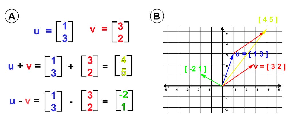
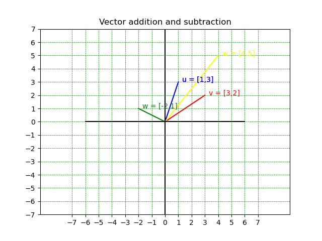
Vector addition and subtraction are fundamental operations in linear algebra. To perform algebraic addition or subtraction of two vectors, we need to ensure that they have the same dimensionality. For instance, we can add two 3-dimensional vectors or two 2-dimensional vectors, but we cannot add a 3-dimensional vector and a 2-dimensional vector (Figure 4A). To add or subtract vectors algebraically, we simply add or subtract the corresponding elements of the vectors. For example, if we have two vectors u and v with components [1, 3] and [3, 2], respectively, then their sum is [4, 5] (Figure 4A).
Geometrically, to add two vectors, we first draw them as arrows with the tail of one vector at the head of the other vector. The sum of the two vectors is the vector that starts at the tail of the first vector and ends at the head of the second vector. The resulting vector represents the displacement between the initial point of the first vector and the final point of the second vector. For instance, suppose we have two vectors u = [1, 3] and v = [3, 2], which are shown in Figure 4B. To add them, we first draw u starting at the origin (0,0) and v starting at the head of u, as shown. The sum of the two vectors is the vector that starts at the origin and ends at the head of v.
In Python, vector addition and subtraction are performed using NumPy arrays.
# Create vectors as NumPy array
u = np.array([1,3])
v= np.array([3,2])

w =u+v  # addition
z=u-v   # subtraction

# plot the vectors
plt.plot([0,u[0]],[0,u[1]], color="blue")
plt.plot([0,v[0]],[0,v[1]], color="red")
plt.plot([0,w[0]],[0,w[1]], color="yellow")
plt.plot([0,z[0]],[0,z[1]], color="green")

plt.axis('equal')
plt.plot([-6, 6],[0, 0],'k-')
plt.plot([0, 0],[-46, 46],'k-')
plt.grid(color = 'green', linestyle = '--', linewidth = 0.5)
plt.axis((-6, 6, -6, 6))
plt.xticks(np.arange(-7, 8, 1))
plt.yticks(np.arange(-7, 8, 1))

plt.title("Vector addition and subtraction")

# Annotate the vector
plt.annotate("u = [1,3]", xy=(1+0.3,3), color ="blue")
plt.annotate("v = [3,2]", xy=(3+0.3,2), color ="red")
plt.annotate("w = [4,5]", xy=(4+0.3,5), color ="yellow")
plt.annotate("w = [-2,1]", xy=(-2+0.3,1), color ="green")

Output:
Vector-Scalar Multiplication
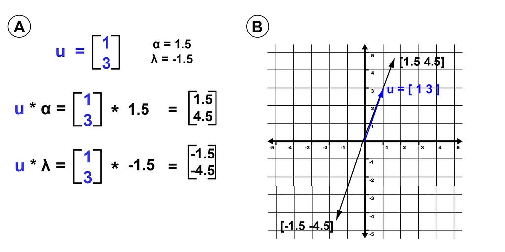
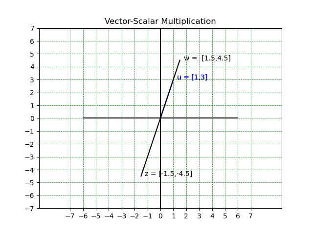
In linear algebra, a scalar refers to a single numerical value, which is not a part of a vector or a matrix. These values (scalars) are commonly represented using lowercase Greek letters like α or λ. Vector-scalar multiplication, denoted as β * u ( u is the vector used throughout this tutorial), is a straightforward operation where each element of the vector is multiplied by the scalar value. This operation results in a new vector with the same direction as the original vector but with a changed magnitude/length (Figure 6B). This scalar multiplication can be used to stretch or shrink vectors, as well as change their direction. For instance, multiplying a vector by a negative scalar (e.g., -1.5) will reverse its direction, while multiplying it by a scalar greater than 1 will stretch it.
In Python, Vector-Scalar Multiplication is performed using the NumPy library.
# Create vectors as NumPy array
u = np.array([1,3])
α=1.5
λ=-1.5

w =u*α
z= u*λ

# plot the vectors
plt.plot([0,u[0]],[0,u[1]], color="blue")
plt.plot([0,w[0]],[0,w[1]], color="black")
plt.plot([0,z[0]],[0,z[1]], color="black")

plt.axis('equal')
plt.plot([-6, 6],[0, 0],'k-')
plt.plot([0, 0],[-46, 46],'k-')
plt.grid(color = 'green', linestyle = '--', linewidth = 0.5)
plt.axis((-6, 6, -6, 6))
plt.xticks(np.arange(-7, 8, 1))
plt.yticks(np.arange(-7, 8, 1))

plt.title("Vector-Scalar Multiplication")
# Annotate the vectors
plt.annotate("u = [1,3]", xy=(1+0.3,3), color ="blue")
plt.annotate("w =  [1.5,4.5]", xy=(1.5+0.3,4.5), color ="black")
plt.annotate("z = [-1.5,-4.5]", xy=(-1.5+0.3,-4.5), color ="black")

Output:
Vector-vector multiplication (dot product)
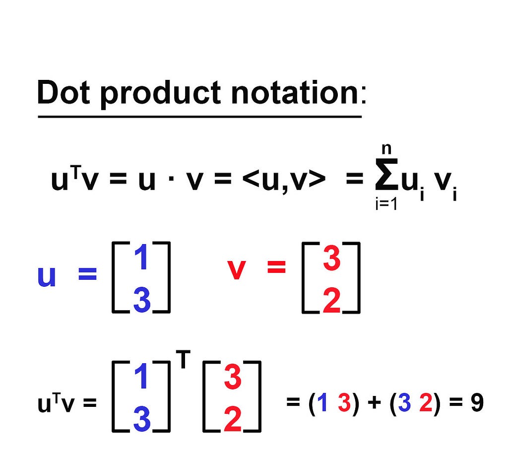
The dot product (also sometimes called the inner product) is one of the most important operations in all of linear algebra. It is the computational building block upon which many algorithms are built, ranging from correlation to convolution to the Fourier transform [2] . The dot product is a single number that provides information about the relationship between two vectors (Figure 8). There are several ways to indicate the dot product between two vectors, the most common notation is uTv (you might also see u · v, <u,v>).
There are multiple ways to implement the dot product in Python.
# Create vectors as NumPy array
u = np.array([1,3])
v= np.array([3,2])

# method 1, using np.dot()
dotp1= np.dot(u,v)

# method 2 using np.matmul()
dotp2= np.matmul(u,v)

# method 3
dotp3= np.sum(np.multiply(u,v))

print(dotp1, dotp2, dotp3)
Output:
9 9 9
The dot product is often viewed as a way to measure the similarity or mapping between two vectors. For example, if we had collected height and weight data from hundreds of people and stored them in two vectors, a large dot product between those two vectors would indicate that the variables are related to each other (e.g., taller people tend to weigh more). However, the magnitude of the dot product is affected by the scale of the data, meaning that the dot product between data measured in different units would not be directly comparable. To address this issue, a normalization factor can be applied, which leads to the normalized dot product known as the Pearson correlation coefficient (“we will cover it in a future tutorial). This coefficient is widely used in statistics and data science and is considered one of the most important analyses in the field [1].
Conclusion
In conclusion, vectors have a significant role in many fields such as mathematics, data science, and engineering. They can be interpreted both algebraically and geometrically, making them essential for useful computations and transformations. The concepts discussed in this tutorial, such as vector magnitude, unit vectors, vector addition and subtraction, and scalar and vector multiplication, are the building blocks of more advanced topics in linear algebra and data analysis. Mastering these concepts can provide you with the necessary skills and tools to solve complex problems in fields such as machine learning, computer vision, and physics.
I have prepared a code review to accompany this blog post, which can be viewed in my GitHub.

References
[1] M. Cohen, Practical Linear Algebra for Data Science: From Core Concepts to Applications Using Python, 1st edition. O’Reilly Media, 2022.
[2] G. Strang, Introduction to Linear Algebra, 6th edition. Wellesley-Cambridge Press, 2023.
[3] “Euclidean distance,” Wikipedia. Apr. 09, 2023. Accessed: Apr. 25, 2023. [Online]. Available: https://en.wikipedia.org/w/index.php?title=Euclidean_distance&oldid=1149051427

Level Up Coding
Thanks for being a part of our community! Before you go:
- 👏 Clap for the story and follow the author 👉
- 📰 View more content in the Level Up Coding publication
- 💰 Free coding interview course ⇒ View Course
- 🔔 Follow us: Twitter | LinkedIn | Newsletter
🚀👉 Join the Level Up talent collective and find an amazing job
Mastering Linear Algebra with Python: An In-Depth Guide to Vectors and Their Applications was originally published in Level Up Coding on Medium, where people are continuing the conversation by highlighting and responding to this story.
This content originally appeared on Level Up Coding - Medium and was authored by MicroBioscopicData
MicroBioscopicData | Sciencx (2023-05-04T16:43:47+00:00) Mastering Linear Algebra with Python: An In-Depth Guide to Vectors and Their Applications. Retrieved from https://www.scien.cx/2023/05/04/mastering-linear-algebra-with-python-an-in-depth-guide-to-vectors-and-their-applications/
Please log in to upload a file.
There are no updates yet.
Click the Upload button above to add an update.