
This content originally appeared on HackerNoon and was authored by Keynesian
:::info Xinyu Li, University of Washington.
:::
Table of Links
- Abstract and Introduction
- 2. Method and 2.1. G is constant
- 2.2. Linear Relation between G and I
- 2.3. Nonlinear Quadratic Relation between G and I
- 3. Results
- 4. Conclusion and References
2. Method
The Keynesian cross model builds upon two ordinary differential equations [6]:
\
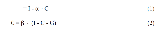
\ where C ≥ 0 is the rate of consumer spending, I ≥ 0 is the national income, and G ≥ 0 is the rate of government spending. The parameters α and β satisfy 1 < α < ∞, 1 ≤ β < ∞. Three relations between government spending and national income are discussed in the following subsections.
2.1. G is constant
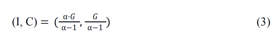
Consider a model consisting of equations (1) and (2) along with a constant government spending G. To determine the equilibrium state for this model, I find the point where = Ċ = 0. Rearranging terms, I obtain the following equilibrium:
\
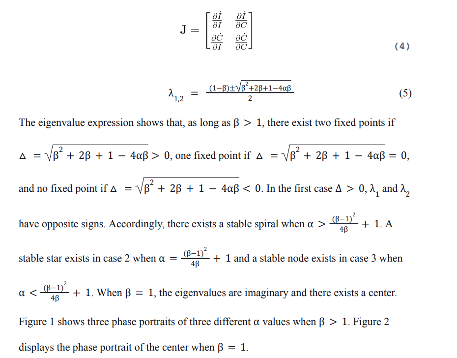
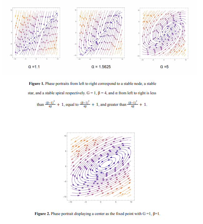
In order to calculate the stability of this fixed point, I compute the Jacobian matrix and eigenvalues:
\
\
:::info This paper is available on arxiv under CC 4.0 license.
:::
\
This content originally appeared on HackerNoon and was authored by Keynesian
Keynesian | Sciencx (2024-07-19T12:00:21+00:00) Bifurcation Analysis of the Keynesian Cross Model: Method and G is constant. Retrieved from https://www.scien.cx/2024/07/19/bifurcation-analysis-of-the-keynesian-cross-model-method-and-g-is-constant/
Please log in to upload a file.
There are no updates yet.
Click the Upload button above to add an update.