
This content originally appeared on Level Up Coding - Medium and was authored by Bhujith Madav Velmurugan

Introduction
The year was 2020, and I had just started dipping my toes into the world of machine learning. Like many beginners, I discovered Natural Language Processing (NLP) and, of course, started with the classic first task: text classification. After starting out with some Udemy tutorials and online resources, I took on my first NLP challenge — the Disaster Tweets Kaggle Competition. Back then, I was using TF-IDF vectorizers to turn text into numbers, followed by scikit-learn classifiers to do the actual classification. Even tiny improvements in performance felt like climbing a mountain.
Fast forward to 2024, and I am working on a similar text classification problem. But now, instead of sweating over every little detail, I just ask GPT-4 to classify the text for me. I often wonder, who was the genius who named Transformers? They truly live up to their name, having transformed the field of AI in ways we could hardly imagine a few years ago. A big shoutout to OpenAI for making AI so accessible. But here is the catch: does this mean we should throw every text classification problem at GPT or other LLMs? Not exactly. Getting these models to work in production is a whole different challenge. Also, the word “Transformers” has pretty much become code for decoder-only LLMs like OpenAI’s GPT or Meta’s LLaMA. However, there is another family of transformer models that quietly powers many NLP applications we use daily, including the likes of Google Search: BERT. These models, particularly their variants, are the unsung heroes behind most NLP applications, especially the ones with semantic search layers, such as Retrieval-Augmented Generation (RAG).
Transformers, have revolutionized NLP, including the humble yet ever-relevant task of text classification. This article is a curated collection of techniques for leveraging transformer models to tackle text classification problems.
For this article, I will be using a multi-label classification dataset to explain various techniques. While there are plenty of resources that cover how to use transformer-based models for binary sequence classification tasks, resources on multi-label classification are surprisingly scarce. This article aims to bridge that gap by discussing some of the techniques for using transformer models in multi-label classification tasks.
Fair warning: No groundbreaking techniques are introduced here. Many of you might already be familiar with the approaches covered. However, during my own exploration of this topic, I noticed a lack of consolidated resources — most articles focus on just one technique. This article is an attempt to organize and present several techniques in one place. I have tried my best to infuse some novelty.
For each technique, I used a variety of transformer models, evaluated their performance using F1 scores, and documented the results. The choice of models, though, was completely random — I admit, there was not much strategy behind it.
The techniques discussed in the article are as follows:
- Classifier using BERT embeddings
- Finetuning transformers with classification heads
- Sentence Transformers Finetuning (SetFit)
- Prompting LLM’s (decoder-only LLM’s)
- Instruction tuning of LLM’s (decoder-only LLM’s)
The article has been structured to provide a high-level overview of each technique, along with the implementation details. I have not delved too deeply into every aspect, but I have included some code snippets to illustrate key points. For the complete code, please refer to this GitHub repository. Additionally, I have shared some personal observations and challenges I encountered while implementing each technique in the form of notes under each section. These insights are meant to help you avoid common pitfalls. However, if any of them are incorrect, please feel free to correct me through your feedback.
Dataset
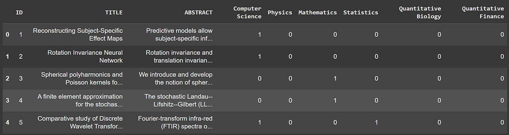
We use a multi-label classification dataset from Kaggle (available at this link) where the goal is to classify research papers into six distinct subjects or labels. Each paper comes with a title and an abstract, and a single paper can belong to more than one subject at the same time.
Before we proceed, it is important to note the distinction between multi-label and multi-class problems. In a multi-class problem, each sample belongs to only one class from a set of multiple classes. In contrast, a multi-label problem allows each sample to belong to multiple classes simultaneously.
Below is a snapshot of how the data looks. It is to be noted that the dataset has class imbalance.

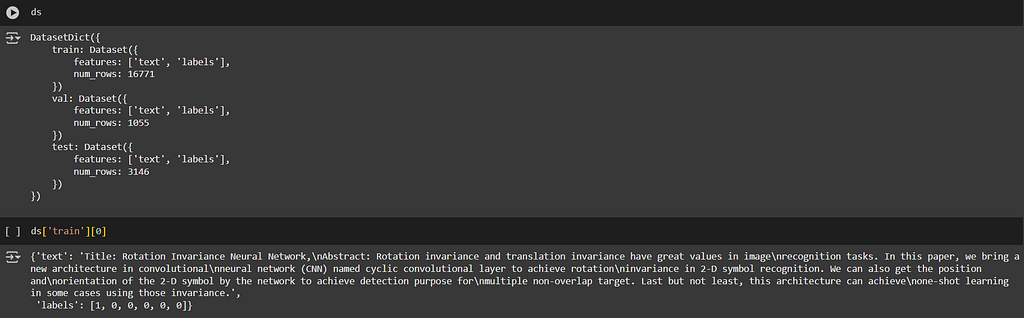
To fine-tune transformer models, we will be using the Hugging Face Transformers library. This library requires the dataset to be in a specific format. Therefore, we’ll preprocess the data by:
- Concatenating the title and abstract into a single input.
- One-hot encoding the labels for compatibility with multi-label classification tasks.
- Splitting the dataset into training, testing, and validation sets.
Finally, convert the processed data into the Hugging Face datasets format to make it ready for fine-tuning. Refer here for the code for processing the dataset.
Let’s start out with our first technique.
1. Classifier using BERT embeddings
n 2018, Google introduced BERT — Bidirectional Encoder Representations from Transformers. How is it different from other transformer models?
The original Transformers paper introduced models with both encoder and decoder components. However, many of the models in the spotlight today, such as GPT and LLAMA, are decoder-only models. These models primarily focus on generating text, and when performing attention — the core mechanism of Transformers — a word cannot “attend” to words on its right. This limitation arises because these models are trained to generate text sequentially, predicting one word at a time.
In contrast, BERT is an encoder-only model. Its key distinction lies in its ability to perform bidirectional attention, meaning it can attend to both the left and right context of a word. This bidirectional nature enables BERT to better understand the meaning of text and produce richer embedding representations. As a result, BERT excels at understanding text rather than generating it, making it ideal for tasks like text classification, sentence similarity, and information retrieval. Today, BERT-style models are widely used for generating sentence embeddings.
To apply BERT in multi-label classification, we leverage its pretrained embeddings and build a classifier on top. But first, we will have a look at how BERT was pretrained.
Key Pretraining Techniques for BERT:
- Masked Language Modeling (MLM):
In this approach, a small percentage of words in the input sentence are randomly masked, and the model learns to predict these masked tokens. Since BERT performs bidirectional attention, it uses both left and right context to predict the masked words. Sentences are tokenized before being fed to the model, and the masked words are replaced with special [MASK] tokens. This training strategy helps BERT generate robust embedding representations. - Next Sentence Prediction (NSP):
Here, the model is trained to predict whether a given pair of sentences logically follows each other. A special [CLS] token is added at the beginning of the sequence, and as the model is trained, this token captures the essence of the entire input sequence.
For our classification task, we use the [CLS] token embeddings as representations of entire sentences. The methodology is straightforward:
- Tokenize the input sentences using BERT’s tokenizer.
- Run the tokenized sentences through the BERT model.
- Extract the embeddings corresponding to the [CLS] token.
- Pass these embeddings as input to a classifier model for prediction.
Instead of solely using the [CLS] token embedding, another approach is to apply max pooling or mean pooling across all token embeddings to create a representation for the entire sentence. Both methods have their pros, and the choice depends on the specific task.

Implementation:
We load the BERT model and its tokenizer using the Hugging Face library. The dataset is tokenized and processed sentence by sentence. For each sentence, we extract the embedding vector corresponding to the [CLS] token — always the first token. This vector serves as input to the classifier.
For this example, I have used a Random Forest Classifier with a OneVsRest wrapper. This wrapper converts the multi-label classification problem into a series of binary classification tasks. In our case, with six labels, the OneVsRest classifier trains six separate Random Forest models, each predicting whether a sample belongs to a specific label.
Of course, this is just one approach. You can experiment with different classifier models, such as logistic regression, support vector machines, or even neural network-based classifiers, to improve performance.
checkpoint = 'google-bert/bert-large-uncased'
config = update_model_related_settings(checkpoint, config)

model, tokenizer = load_model_and_tokenizer(config=config,
                                            add_pad_token=False,
                                            peft=False,
                                            load_model_for_sequence_classification=False
                                            )

ds = tokenize_dataset(tokenizer,
                      config)

f1_score_results, time_taken = build_classifier_using_hidden_states(ds, model, tokenizer)
For the complete code implementation, you can check out here. In my experiments, I used two different BERT model variants to generate embedding representations, which serve as inputs to the Random Forest models.
Results
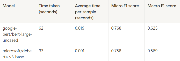
The models were trained on a dataset containing approximately 16,000 examples and tested on a separate dataset of around 3,000 examples. Below are the results of the experiments:
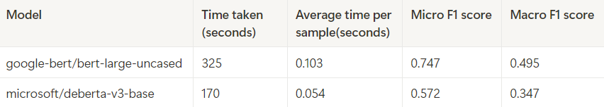
The results show that we achieved respectable F1 scores. As expected, larger models take more time to generate outputs compared to smaller models. All experiments were conducted on Google Colab’s T4 GPU (16GB VRAM). How to interpret these scores ?
- Micro F1 Score: This metric provides insight into the overall model performance across all classes, weighing each instance equally.
- Macro F1 Score: This metric evaluates the model’s performance at the class level by calculating the F1 score for each class and taking their average, treating all classes equally regardless of size.
A higher micro F1 score but a lower macro F1 score suggests that the model performs well overall but struggles with certain classes, likely due to class imbalance in the dataset. We will set these scores as our baseline and explore various techniques to improve them further. The time taken column indicates the time taken to predict 3143 samples in the testing dataset.
2. Finetuning with classification head
This technique is quite similar to the previous one, with the main difference being that here we fine-tune the BERT model. In the previous method, we used a pre-trained model, but when fine-tuning, we adapt the model specifically for a task. Let’s dive into how it’s done.
Hugging Face offers a class called AutoModelForSequenceClassification, which we can instantiate just like other transformer models. So, what’s the difference here? In the previous approach, we took the [CLS] token embeddings and built our own classifier on top. With fine-tuning, Hugging Face does the heavy lifting for us. A classification head is attached to the top of the [CLS] token, taking the embedding vector and outputting logits corresponding to the number of classes (in this case, 6).
You might wonder, what happens if we’re using decoder-only models like LLAMA, which don’t have a [CLS] token? In such cases, the last token — typically the one that attends to all previous tokens in the sequence (note that decoder-only models don’t have bidirectional attention) — serves as input to the classifier.

When fine-tuning BERT, we adjust the model for our specific task. Hugging Face simplifies this process with its Trainer library, which streamlines fine-tuning.
Implementation
The following code block loads the tokenizer and transformer models with a classification head attached, based on the model name. For this experiment, we fine-tuned the models using the QLORA technique, which involves loading a quantized version of the model and then fine-tuning a small set of parameters, called an adapter, placed on top of the model (LORA). For this setup, I have used models quantized to 4 bits.
With LORA, we have the flexibility to decide on which weight matrices the adapters should be attached to. One thing to note is that the weights of the LORA adapter will be of type bf16 or fp16 while we have quantized the weights of the base model to 4 bits. This has to be taken care during inference.
In this experiment, I fine-tuned 5 different models: 2 encoder-only models and 3 decoder-only models. The decoder-only models were fine-tuned using QLORA, while the encoder-only models were fine-tuned fully. All models were fine-tuned on A40 GPUs (48GB VRAM, 50GB RAM) hosted by RunPod.
Note:
- Encoder-only models typically come with a default pad token, while for decoder-only models, the pad token must be manually added.
tokenizer = AutoTokenizer.from_pretrained(config.checkpoint)
add_pad_token = True
peft = True

# Llama version 3 models already have a padding token
# Hence we need not add a padding token
if add_pad_token:
    if 'Llama' in tokenizer.name_or_path:
        tokenizer.pad_token = '<|finetune_right_pad_id|>'
    else:
        tokenizer.add_special_tokens({"pad_token":"<pad>"})

# I faced some errors while right padding in Mistral models
# Hence set padding_side as left for Mistral models alone
if 'Mistral' in tokenizer.name_or_path:
    tokenizer.padding_side = "left"
else:
    tokenizer.padding_side = "right"

    if load_model_for_sequence_classification:

# Load the model with classification head
# num_labels specifies the number of neurons in the output layer
model =  AutoModelForSequenceClassification.from_pretrained(
  pretrained_model_name_or_path=config.checkpoint,
  quantization_config=quantization_config(config) if quantization else None,
  torch_dtype=torch.bfloat16 if config.bf16 else torch.float16,
  num_labels=config.num_labels,
  problem_type=config.problem_type
)

if add_pad_token:
    model.config.pad_token_id = tokenizer.pad_token_id
    if 'Llama' not in tokenizer.name_or_path:
        model.resize_token_embeddings(len(tokenizer))
if peft:
    peft_config = LoraConfig(
        task_type=TaskType.SEQ_CLS,
        r=config.lora_rank,
        lora_alpha=config.lora_alpha,
        lora_dropout=config.lora_dropout,
        bias=config.lora_bias,
        #target_modules=["q_proj", "k_proj"]
    )

    model = get_peft_model(model, peft_config)
The code block below demonstrates how the model can be fine-tuned. There are many resources that explain the QLORA fine-tuning technique in detail, along with the various parameters involved. For the complete code, please refer here. The parameter values used here were selected based on those commonly found in most tutorials and resources.
Note:
If you encounter out of memory errors, try reducing the train_batch_size. Additionally, setting bf16=True during fine-tuning can help speed up the training process. However, note that this feature is only available on the latest GPUs.
num_train_epochs = config.num_train_epochs
train_batch_size = config.batch_size
gradient_accumulation_steps = config.gradient_accumulation_steps
max_steps = int((len(ds['train'])*num_train_epochs)/(train_batch_size*gradient_accumulation_steps))

training_args = TrainingArguments(
    output_dir=f"./{config.model_name}_results",
    max_steps=max_steps,
    learning_rate=3e-5,
    lr_scheduler_type="cosine",
    optim="paged_adamw_32bit",
    per_device_train_batch_size=train_batch_size,
    per_device_eval_batch_size=train_batch_size,
    gradient_accumulation_steps=gradient_accumulation_steps,
    gradient_checkpointing=config.gradient_checkpointing,
    weight_decay=0.01,
    warmup_ratio=0.1,
    evaluation_strategy="steps",
    save_strategy="epoch",
    logging_strategy="steps",
    logging_steps=100,
    save_steps=max_steps-100,
    eval_steps=100,
    report_to="wandb",
    run_name=f"{config.repo_user_id}/{config.model_name}_results",
    fp16=config.fp16,
    bf16=config.bf16
)

trainer = Trainer(
    model=model,
    tokenizer=tokenizer,
    args=training_args,
    train_dataset=ds["train"],
    eval_dataset=ds["val"],
    compute_metrics=compute_metrics
)

trainer.train()

trainer.model.save_pretrained(config.local_save_path)
The following code can be used to upload the model to the Hugging Face repository. The fine-tuned adapter model is obtained using trainer.model, and this model is then uploaded to the Hugging Face repository. The load_model_and_tokenizer function loads the quantized version of the base model (including the classification head) and the tokenizer with pad tokens added. The PeftModel.from_pretrained and merge_and_unload() functions take the base model, attach the fine-tuned adapter, and then merge the adapter weights into the base model. Finally, the model and tokenizer are pushed to the Hugging Face repository, making the fine-tuned model accessible for others.
Note:
It is crucial to load the model with the same quantization configuration that was used during fine-tuning. If you load a pre-trained model without the correct quantization settings and attach an adapter fine-tuned with a quantized pre-trained model, the model’s performance may degrade.
trainer.model.push_to_hub(f"{config.repo_user_id}/{config.model_name}_adapter", safe_serialization=True, max_shard_size='3GB')
base_model, tokenizer = load_model_and_tokenizer(config,
                                                 quantization=quantized,
                                                 add_pad_token=add_pad_token,
                                                 peft=False,
                                                 load_model_for_sequence_classification=True)
model = PeftModel.from_pretrained(model=base_model, model_id=f"{config.repo_user_id}/{config.model_name}_adapter")
model = model.merge_and_unload()

model.push_to_hub(f"{config.repo_user_id}/{config.model_name}", safe_serialization=True, max_shard_size='3GB')
tokenizer.push_to_hub(f"{config.repo_user_id}/{config.model_name}")
The below code can be used for inference.
checkpoint = "bhujith10/Mistral-7B-Instruct-v0.3_finetuned_with_classification_head_2024_12_26_08_34"

model =  AutoModelForSequenceClassification.from_pretrained(
            pretrained_model_name_or_path=checkpoint,
            use_cache=True,
            torch_dtype=torch.bfloat16 if config.bf16 else torch.float16,
            num_labels=config.num_labels,
            problem_type=config.problem_type
        )

tokenizer = AutoTokenizer.from_pretrained(checkpoint)

ds_tokenized = tokenize_dataset(tokenizer, config, dataset_name='bhujith10/multi_class_classification_dataset')

# DataLoader for batching
batch_size = 4
dataloader = DataLoader(ds_tokenized['test'], batch_size=batch_size)

predicted_labels = []
actual_labels = []

# Generate for each batch
start_time = time.time()
for i,inputs in enumerate(dataloader):
    print(f"Batch {i}")
    batch = {key: inputs[key].to('cuda') for key in ['input_ids','attention_mask']}

    actual_labels.extend(list(i) for i in inputs['labels'].detach().to(torch.int8).numpy())

    outputs = model(**batch)

    logits_array = outputs.logits.detach().cpu().to(torch.float16).numpy()

    tmp_predicted_labels = [list(return_encodings(arr)) for arr in logits_array]
    predicted_labels.extend(tmp_predicted_labels)

end_time = time.time()
print('total time ',end_time - start_time)
Results
The results of the technique are shown below.
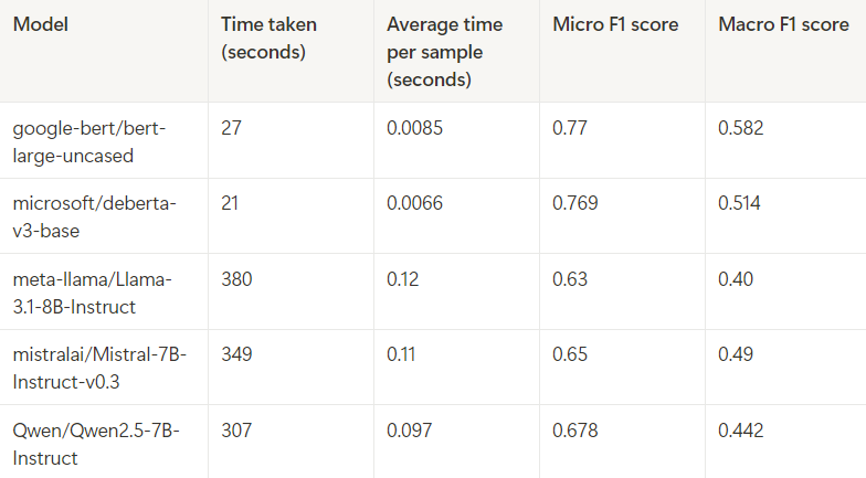
All models were trained for only 1 epoch, and the dataset size remained consistent with the first technique. I was a bit surprised by the results. I had expected the decoder-only models like Llama and Mistral to outperform the encoder-only models. However, the results were the opposite. The bert-large-uncased model ended up being the top performer.
Notes:
- I initially tried training the Llama 8B model for multiple epochs in an attempt to increase the F1 scores, but there was no significant improvement. I assumed that this trend would hold true for other decoder-only models as well.
- However, when I increased the dataset size — regardless of the model — I observed a notable improvement in the metrics. Initially, I had started with only half of the dataset for training, which resulted in suboptimal F1 scores. But as I increased the dataset size, the F1 scores improved significantly.
3. Sentence Transformers Fine Tuning (SetFit)
“SetFit is a model framework to efficiently train text classification models with surprisingly little training data.” This technique closely mirrors the previous approach. In the second technique, we added a classification head on top of transformers and fine-tuned them. Here, we follow a similar approach. The key difference lies in how the models are fine-tuned.
The Sentence Transformers library and SBERT (Sentence-BERT), introduced in 2019, addressed challenges in tasks like sentence similarity and semantic search. While SBERT models and the Sentence Transformers library are related, they are not the same. For a detailed explanation, refer to this article. To summarize:
To obtain sentence embeddings using BERT, one would typically extract embeddings corresponding to the CLS token or perform mean pooling on individual token embeddings. The Sentence Transformers library simplifies this process by handling these steps internally and directly returning the sentence embedding representation.
The significant distinction between the original BERT models and SBERT models lies in their training. SBERT models are fine-tuned BERT models trained in a siamese architecture using contrastive pairs of sentences. This training enables SBERT models to generate similar embeddings for semantically similar sentences. For instance, the original SBERT model was fine-tuned on the Stanford NLI dataset.
Now that we have grasped the essence of SBERT models, let us discuss SetFit. As the name suggests, SetFit combines a sentence transformer model with a classification head. The idea is to fine-tune the sentence transformer model to generate embeddings specifically useful for our classification task.
SetFit employs contrastive learning for fine-tuning. You might wonder: What if we do not have contrastive sentence pairs, which are core to SBERT’s training? This is where the SetFit framework shines. It generates synthetic contrastive pairs to enable fine-tuning without requiring pre-existing contrastive data.
Example: Contrastive Pairs for Fine-Tuning
Let’s illustrate this with an example generated using ChatGPT. Assume we have the following:
Positive Sentences:
- The sky is blue.
- The grass is green.
- The sun is bright.
Negative Sentences:
- The sky is not blue.
- The grass is not green.
- The sun is not bright.
Using these sentences, we create similar pairs (positive-positive) and dissimilar pairs (positive-negative):
Positive-Positive Pairs:
- (The sky is blue, The grass is green)
- (The sky is blue, The sun is bright)
- (The grass is green, The sun is bright)
Positive-Negative Pairs:
- (The sky is blue, The sky is not blue)
- (The sky is blue, The grass is not green)
- (The sky is blue, The sun is not bright)
- (The grass is green, The sky is not blue)
- (The grass is green, The grass is not green)
- (The grass is green, The sun is not bright)
- (The sun is bright, The sky is not blue)
- (The sun is bright, The grass is not green)
- (The sun is bright, The sun is not bright)
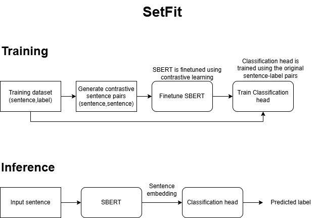
In a similar way, given a dataset, SetFit generates contrastive sentence pairs. During fine-tuning, sentences with the same label are embedded closer together in the vector space, while sentences with different labels are embedded further apart.
What About the Classification Head? By default, SetFit uses a logistic regression classifier as the classification head. However, there is flexibility to use neural networks or custom classification heads depending on the use case. It is worth noting that when training the classification head, the labeled samples from the dataset are used directly — not the contrastive sentence pairs. For multi-class classification tasks, SetFit supports all strategies provided by scikit-learn, ensuring compatibility with a wide range of classification techniques.
Implementation
The following code snippet demonstrates how to fine-tune using SetFit. Pay attention to the num_epochs parameter in TrainingArguments. This parameter is defined as a tuple (1, 16). Here:
- The first integer (1) specifies the number of epochs for fine-tuning the transformer model.
- The second integer (16) determines the number of epochs for training the classification head.
Note:
In the example shown above, we had only two classes, and the number of pairs was limited. However, as the number of classes and the number of sentences per class increase, the number of generated pairs grows exponentially. Hence, I had selected a small subset of the dataset for fine-tuning.
labels=['Computer Science', 'Physics', 'Mathematics', 'Statistics', 'Quantitative Biology', 'Quantitative Finance']

tmp_train_dataset = train_dataset.select(range(150)).shuffle()
tmp_eval_dataset = eval_dataset.select(range(50)).shuffle()

# Load a SetFit model from Hub
model = SetFitModel.from_pretrained(
    model_id="google-bert/bert-large-uncased",
    multi_target_strategy="one-vs-rest",
    use_differentiable_head=True,
    head_params={"out_features": len(labels)},
    labels=labels
)

model.to('cuda')

args = TrainingArguments(
    batch_size=4,
    num_epochs=(1,16),
    eval_strategy="epoch",
    save_strategy="epoch",
    load_best_model_at_end=True
)

trainer = Trainer(
    model=model,
    args=args,
    train_dataset=tmp_train_dataset,
    eval_dataset=tmp_eval_dataset,
    metric="accuracy",
    column_mapping={"text": "text", "labels": "label"}
)

# Train and evaluate
trainer.train()

trainer.model.save_pretrained("bert-large-uncased-setfit_finetuned")
I experimented with two models, and the results are shown below. Both models were trained for 1 epoch, using only 150 samples for training. The training was conducted on an A40 GPU. Notably, the macro F1 scores surpassed those achieved in the second technique, demonstrating the effectiveness of this approach even with a limited dataset. You can try finetuning with different models or with a different loss function to check for possible improvements. I had used the default cosine similarity loss . Refer here for the code implementation.
Results
Two different BERT models were finetuned using the SetFit framework and we have acheived a significant improvement in the macro F1 scores compared to the earlier techniques, especially in case of bert-large-uncased model. Micro F1 score remains almost same compared to the previous techniques.
4. Prompting LLM’s (decoder-only LLM’s)
This technique would be the simplest of all techniques. Just prompt the decoder-only models to classify the text. That’s it. But it is not that simple. All these billion parameter models are very effective in generating human like text. The problem is the non-deterministic nature of these models. The same model prompted with the same message twice has a high chance of returning two different outputs.
Large Language Models (LLMs) are trained on extensive datasets, often encompassing a significant portion of the web. As a result, they have a high likelihood of accurately classifying research papers into their respective subjects. However, the real challenge lies in ensuring that the LLM generates the labels in the exact format we need for downstream tasks.
Fortunately, with OpenAI’s Structured Outputs feature, we can confidently ensure that models like GPT-4o (and later versions) produce outputs consistently in the desired format. This eliminates much of the ambiguity and variability associated with free-form responses.
Implementation
The code block below demonstrates how to utilize the GPT-4o model to generate outputs in the required structured format:
def classify(sample, client, temperature=0.6, top_p=0.0):
    """
    Classifies the title of a research paper into one or more predefined subjects.

    Parameters
    ==========
    sample (dict): A dictionary containing a key 'text' with the title of the research paper.
    client (OpenAI): An instance of the OpenAI client to generate predictions.
    temperature (float): Sampling temperature for the model.
    top_p (float): Top-p sampling value for nucleus sampling.

    Returns
    =======
    dict: The input `sample` dictionary augmented with a 'Predictions' key containing the predicted subjects.
    """

    # Define the schema for the structured response format
    # Returns a list of predicted subjects
    class classify_research_paper(BaseModel):
        Subjects: list[str]

    # Instruction prompt
    system_msg = """Given the title of a research paper, classify it into one or more of the following subjects based on the content: ['Computer Science', 'Physics', 'Mathematics', 'Statistics', 'Quantitative Biology', 'Quantitative Finance'].

    Return only the list with only the most appropriate subjects (1-3) from the list.
    Do not include subjects outside the provided list.
    Avoid selecting all subjects. Select subjects most relevant to the content.
    """

    messages = [
        {"role": "system", "content": system_msg},
        {"role": "user", "content": sample['text']}
    ]

    # Call the OpenAI API for classification
    completion = client.beta.chat.completions.parse(
        model=os.getenv("MODEL"),
        messages=messages,
        response_format=classify_research_paper,
        temperature=temperature,
        top_p=top_p
    )

    # Extract and parse the response
    response_content = completion.choices[0].message.parsed
    response = json.loads(response_content)

    # Add the predicted subjects to the sample
    sample['Predictions'] = response['Subjects']

    return sample

# Initialize the OpenAI client
client = OpenAI()

try:
    dataset = load_dataset('bhujith10/multi_class_classification_dataset', split="test")
except Exception as e:
    raise RuntimeError(f"Error loading dataset: {e}")

# Apply the classification function to each entry in the dataset
dataset_with_predictions = dataset.map(lambda sample: classify(sample, client))
Refer here for the code. The raw responses from the GPT model could be found here. The predicted subjects were converted into encodings, and the F1 scores were calculated and recorded. These scores are summarized in the table below.
While the proprietary model performed well, let’s explore how open-source decoder-only models, like those used in the second technique, compare. To maintain uniformity, I used the same prompt with only minor adjustments. However, a key limitation of open-source LLMs is the lack of assurance for structured outputs. Hence, I have added an example input and output to the prompt to ensure some reliability. Even then we can’t be assured that the LLM will adhere to this particular format.
To address this, I generated the responses and extracted the predictions list using regex patterns. The code for this process is shown below. Before prompting the LLMs, we format the text in a specific structure and tokenize it before feeding it to the model. The inputs are then batched, and inference is run in batches to calculate processing time.
Each LLM has its own prompt templates and special tokens. By importing the tokenizers from HuggingFace, we can also access the chat template for a particular model using the apply_chat_template function. This function defines how to convert conversations (represented as lists of messages) into a single tokenizable string in the format the model expects.
Note:
In the code below, there is a slight variation for Mistral models. The system prompt was not being added to the message when the chat template was applied. To address this, the system prompt was explicitly included.
def format_text_for_inference(sample, tokenizer):
    """
    Formats the input sample for inference by constructing a chat-like template.

    Parameter
    =========
    sample (dict): A dictionary containing the 'text' key with the title and abstract of the research paper.
    tokenizer: The tokenizer object used to preprocess and format the text.

    Returns
    =======
    dict: The input sample augmented with a 'formatted_text' key containing the processed text.
    """

    # Instruction prompt
    system_content = f"""
    Given the title and abstract of a research paper, classify it into one or more of the following subjects based on its content: ['Computer Science', 'Physics', 'Mathematics', 'Statistics', 'Quantitative Biology', 'Quantitative Finance'].

    Output Requirements:

    Return only the most appropriate subjects (1 to 3) from the given list.
    Do not include subjects outside the provided list.
    Avoid selecting all subjects; focus on those most relevant to the paper's content.
    You are provided with an example

    RETURN ONLY A LIST AND NOTHING ELSE
    """

    # The actual text for classification
    user_content = sample['text']

    # Input and output for better context to the model
    example_user_input = f"""
    Title: Efficient methods for computing integrals in electronic structure calculations,
    Abstract: Efficient methods are proposed, for computing integrals appearing in electronic structure calculations.
    The methods consist of two parts: the first part is to represent the integrals as contour integrals and the second one is to evaluate the contour integrals by the Clenshaw-Curtis quadrature.
    The efficiency of the proposed methods is demonstrated through numerical experiments.
    """
    example_user_output = f"""
    ['Physics']
    """

    # Handle different tokenizer types
    if 'mistralai' in tokenizer.name_or_path:
        # For Mistral tokenizers
        user_content = system_content + "\n" + example_user_input + "\n" + example_user_output + "\n" + user_content
        messages = [
            {
                "role": "user",
                "content": user_content
            }
        ]
    else:
        # For other tokenizers, use a different template
        messages = [
            {
                "role": "system",
                "content": system_content,
            },
            {
                "role": "user",
                "content": example_user_input
            },
            {
                "role": "assistant",
                "content": example_user_output
            },
            {
                "role": "user",
                "content": user_content
            }
        ]

    # Apply the chat template to the sample using the tokenizer
    sample["formatted_text"] = tokenizer.apply_chat_template(messages, tokenize=False)

    return sample
Refer here for the code implementation for prompting open source models. The raw responses from the pre-trained model and finetuned model are stored as csv files here.
Results
The metrics obtained from using different models are summarized below. Each model was tasked with generating up to 256 tokens (excluding the input tokens) for every input. Unfortunately, the results were not very impressive overall. While Mistral and Qwen models performed reasonably well, Llama was lagging behind. But none of the models could match the performance of GPT model.

The subpar results could be due to one of two reasons:
- The model failed to produce responses in the desired format.
- The model returned responses in the correct format, but the predictions were inaccurate.
To further investigate, we need to analyze the model responses more granularly. The table above provided metrics for all samples in the dataset, regardless of whether the model responses included the predicted subjects list. However, the table below focuses solely on responses that contained the predicted subjects list in the desired format.
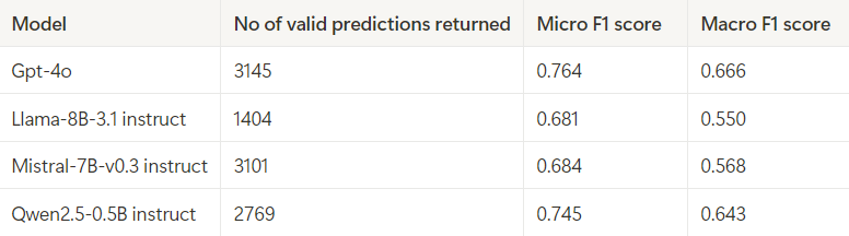
Mistral emerged as the most reliable performer among open-source models, returning correctly formatted responses over 90% of the time. For all models, the F1 scores calculated for these valid responses showed a noticeable improvement compared to the overall dataset metrics.
The analysis indicates that the primary challenge lies in ensuring the responses are returned in the desired format, rather than in the accuracy of the predictions themselves. Can we tailor the LLMs to reliably return outputs in our desired format? This will be explored in the next technique.
5. Instruction Tuning LLM’s (decoder-only LLM’s)
The last technique involves fine-tuning open-source LLMs to generate responses in the desired format. While foundational LLMs are highly generalized, specific use cases like ours require specialized models tailored to perform particular tasks effectively. This approach, known as instruction tuning, aligns the model’s outputs with the task requirements.
GPT models — the core of ChatGPT — are decoder-only models trained to generate text by predicting the next token based on input text. Through instruction tuning, these models were fine-tuned using datasets containing instructions paired with examples of inputs and desired outputs. This step enabled the models to better understand and respond to task-specific prompts. Further refinement was achieved via reinforcement learning with human feedback (RLHF), which taught the models to generate responses that align with human preferences, ultimately elevating GPT to the ChatGPT level.
Similarly, companies like Meta or Mistral release instruction-tuned versions of their foundational LLM models which offers improved task-specific performance. The name instruction tuning reflects the way datasets are constructed — by pairing instructions with corresponding outputs. For example, in our case, the dataset will include prompts with instruction and the actual labels in the desired format. This supervised fine-tuning ensures that the models produce consistent and reliable outputs.
Implementation
This approach might appear similar to the prompt used in the previous technique, but the key difference is that it now contains both the instruction and the corresponding answer. In essence, the model is trained to follow a specific pattern — taking an instruction and generating an output that aligns with the desired format.
In the below code, I have shown an example of how the text and label is formatted to fit instruction tuning.
Text:
  Title: Rotation Invariance Neural Network,
  Abstract: Rotation invariance and translation invariance have great values in image
  recognition tasks. In this paper, we bring a new architecture in convolutional
  neural network (CNN) named cyclic convolutional layer to achieve rotation
  invariance in 2-D symbol recognition. We can also get the position and
  orientation of the 2-D symbol by the network to achieve detection purpose for
  multiple non-overlap target. Last but not least, this architecture can achieve
  one-shot learning in some cases using those invariance.

label:
  [1, 0, 0, 0, 0, 0]

Subject:
  ['Computer Science']

Formatted Text:
<|begin_of_text|><|start_header_id|>system<|end_header_id|>

Cutting Knowledge Date: December 2023
Today Date: 26 Jul 2024

Given the title and abstract of a research paper, classify it into one or more of the following subjects based on its content: ['Computer Science', 'Physics', 'Mathematics', 'Statistics', 'Quantitative Biology', 'Quantitative Finance'].

    Output Requirements:

    Return only the most appropriate subjects (1 to 3) from the given list.
    Do not include subjects outside the provided list.
    Avoid selecting all subjects; focus on those most relevant to the paper's content.

    RETURN ONLY A LIST AND NOTHING ELSE<|eot_id|><|start_header_id|>user<|end_header_id|>

Title: Efficient methods for computing integrals in electronic structure calculations,
    Abstract: Efficient methods are proposed, for computing integrals appeaing in electronic structure calculations.
    The methods consist of two parts: the first part is to represent the integrals as contour integrals and the second one is to evaluate the contour integrals by the Clenshaw-Curtis quadrature.
    The efficiency of the proposed methods is demonstrated through numerical experiments.<|eot_id|><|start_header_id|>assistant<|end_header_id|>

['Physics']<|eot_id|><|start_header_id|>user<|end_header_id|>

Title: Rotation Invariance Neural Network,
Abstract: Rotation invariance and translation invariance have great values in image
recognition tasks. In this paper, we bring a new architecture in convolutional
neural network (CNN) named cyclic convolutional layer to achieve rotation
invariance in 2-D symbol recognition. We can also get the position and
orientation of the 2-D symbol by the network to achieve detection purpose for
multiple non-overlap target. Last but not least, this architecture can achieve
one-shot learning in some cases using those invariance.<|eot_id|><|start_header_id|>assistant<|end_header_id|>

['Computer Science'] <|end_of_text|><|eot_id|>
The below code shows how the entire dataset can be formatted using the apply_chat_template function we had discussed in the previous module.
def format_text(sample, tokenizer):
  """
  Formats the input sample for a language model using a chat-based template.
  It includes system instructions, an example interaction, and the user's input.

  Parameters
  ==========
  sample (dict): A dictionary containing the sample data, including 'text' (title and abstract) and 'labels'.
  tokenizer: A tokenizer object used for formatting text for language model input.

  Returns
  =======
  dict: The updated sample dictionary with the formatted text added as 'formatted_text'.
  """
  system_content = """
  Given the title and abstract of a research paper, classify it into one or more of the following subjects based on its content: ['Computer Science', 'Physics', 'Mathematics', 'Statistics', 'Quantitative Biology', 'Quantitative Finance'].

  Output Requirements:

  Return only the most appropriate subjects (1 to 3) from the given list.
  Do not include subjects outside the provided list.
  Avoid selecting all subjects; focus on those most relevant to the paper's content.

  RETURN ONLY A LIST AND NOTHING ELSE
  """
  user_content = sample['text']

  example_user_input = f"""
  Title: Efficient methods for computing integrals in electronic structure calculations,
  Abstract: Efficient methods are proposed, for computing integrals appeaing in electronic structure calculations.
  The methods consist of two parts: the first part is to represent the integrals as contour integrals and the second one is to evaluate the contour integrals by the Clenshaw-Curtis quadrature.
  The efficiency of the proposed methods is demonstrated through numerical experiments.
  """
  example_user_output=f"""
  ['Physics']
  """

  if 'mistralai' in tokenizer.name_or_path:

      assistant_content = str(return_subjects(sample['labels'])) + '\t' + tokenizer.eos_token

      user_content = system_content + "\n" + example_user_input + "\n" + example_user_output + "\n" + user_content

      messages = [
          {
              "role": "user",
              "content": user_content
          },
          {
              "role":"assistant",
              "content":assistant_content
          }
      ]

  else:
      assistant_content = str(return_subjects(sample['labels'])) + '\t' + '<|end_of_text|>'
      messages = [
          {
              "role": "system",
              "content": system_content,
          },
          {
              "role": "user",
              "content": example_user_input
          },
          {
              "role": "assistant",
              "content": example_user_output
          },
          {
              "role": "user",
              "content": user_content
          },
          {
              "role":"assistant",
              "content":assistant_content
          }
      ]


  sample["formatted_text"] = tokenizer.apply_chat_template(messages, tokenize=False)

  return sample
I fine-tuned three open-source models using the QLORA technique for one epoch, leveraging an instruction dataset with approximately 4,000 samples. This process was followed by extracting predictions from the responses and calculating the F1 scores between the actual and predicted labels. OpenAI also supports fine-tuning of GPT models. However, it comes with its own costs, which is why I have not tried it. The below code block shows how the models can be finetuned.
tokenizer = AutoTokenizer.from_pretrained(config.checkpoint, add_prefix_space=True)

# Configure tokenizer for specific models
if 'Llama' in config.checkpoint:
    # Set the pad token and padding side for Llama model
    tokenizer.pad_token='<|finetune_right_pad_id|>'
    tokenizer.padding_side = 'right'
else:
    # Add a pad token and set padding side for non-Llama models
    tokenizer.add_special_tokens({"pad_token":'<pad>'})
    tokenizer.padding_side = 'left'

# Load the pre-trained causal language model
model = AutoModelForCausalLM.from_pretrained(
    config.checkpoint,
    attn_implementation="flash_attention_2",
    use_cache=False, # Disable KV cache during finetuning
    device_map=config.device_map,
    quantization_config=quantization_config(config) if quantization else None,
    torch_dtype=torch.bfloat16 if config.bf16 else torch.float16,
    trust_remote_code=True
)

model.config.pad_token_id = tokenizer.pad_token_id

# Resize token embeddings for non Llama models to account for additional tokens
if 'Llama' not in config.checkpoint:
    model.resize_token_embeddings(len(tokenizer))

# Calculate the maximum number of training steps
num_train_epochs = config.num_train_epochs
train_batch_size = config.batch_size
gradient_accumulation_steps = config.gradient_accumulation_steps
max_steps = int((len(dataset['train'])*num_train_epochs)/(train_batch_size*gradient_accumulation_steps))

if peft:
    # Load LoRA configuration
    peft_config = LoraConfig(
        r=config.lora_rank,
        lora_alpha=config.lora_alpha,
        lora_dropout=config.lora_dropout,
        bias=config.lora_bias,
        task_type="CAUSAL_LM",
        #target_modules=["q_proj", "k_proj", "v_proj", "o_proj"]
    )

training_arguments = SFTConfig(
    max_steps=max_steps,
    per_device_train_batch_size=train_batch_size,
    gradient_accumulation_steps=gradient_accumulation_steps,
    gradient_checkpointing=True,
    learning_rate=3e-4,
    fp16=config.fp16,
    bf16=config.bf16,
    output_dir=f"{config.model_name}_outputs",
    optim="paged_adamw_32bit",
    eval_steps=100,
    save_steps=max_steps-100,
    logging_steps=100,
    save_strategy="steps",
    evaluation_strategy="steps",
    warmup_ratio=0.02,
    report_to="wandb",
    run_name=f"{config.repo_user_id}/{config.model_name}_results",
    lr_scheduler_type="cosine",
    dataset_batch_size=4,
    max_seq_length=config.max_length,
    dataset_text_field=dataset_text_field
)

# Set supervised fine-tuning parameters
trainer = SFTTrainer(
      model=model,
      peft_config=peft_config,
      train_dataset=dataset["train"],
      eval_dataset=dataset["val"],
      tokenizer=tokenizer,
      args=training_arguments
)

trainer.train()

trainer.model.save_pretrained(config.local_save_path)
In the earlier fine-tuning technique, increasing the size of the dataset led to significant improvements in metrics. However, in this case, increasing the number of samples did not enhance the quality of the results. In fact, the models fine-tuned on the entire dataset of 16,000 samples generated nearly identical responses for every text, indicating that they started to overfit.
Refer here for the complete code.
Note:
In the case of instruction fine-tuning, my observation is that we might not require a large number of samples. Please correct me if my observation is not correct.
Results
Results of the instruction tuning is shown below.

I finally had my Eureka moment! After all the efforts involved in fine-tuning these models, Mistral-7B-Instruct-v0.3 has produced the best metrics. We have even outperformed OpenAI. Now, lets determine whether instruction tuning has improved the number of valid responses — i.e., responses containing the predicted subjects list.
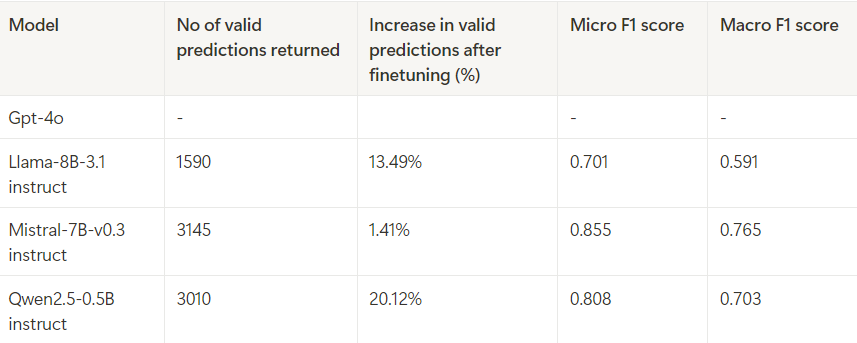
Instruction tuning has definitely elevated the quality of responses compared to the previous technique. In fact, Mistral has delivered the desired response 100% of the time.
Conclusion
We have discussed five different techniques for tackling multi-class classification problems, and I’ve aimed to provide as much clarity as possible for each approach. My intention was to make this article a comprehensive resource for using transformers in classification tasks. Writing this has been a rewarding learning experience for me, and I hope it proves equally insightful for you. If not, I sincerely apologize.
Thanks a lot for reading. I would greatly appreciate your feedback.
My sincere and heartfelt thanks to Ashish Vaswani, Noam Shazeer, Niki Parmar, Jakob Uszkoreit, Llion Jones, Aidan N. Gomez, Lukasz Kaiser, Illia Polosukhin. These individuals have no direct connection to this article, but without their contributions, this article might not have existed.
Codebase and Model artifacts
The complete code is available at https://github.com/Bhujith10/Multi-Label-Classification-using-Transformers.git
The finetuned models and HuggingFace datasets can be accessed at https://huggingface.co/bhujith10
Key resources that helped me
Natural Language Processing with Transformers — https://www.oreilly.com/library/view/natural-language-processing/9781098136789/
LLM Course — https://github.com/mlabonne/llm-course
Lora for sequence classification with Roberta, Llama, and Mistral — https://github.com/mehdiir/Roberta-Llama-Mistral
How We Scaled Bert To Serve 1+ Billion Daily Requests on CPUs
Text Classification in the era of Transformers was originally published in Level Up Coding on Medium, where people are continuing the conversation by highlighting and responding to this story.
This content originally appeared on Level Up Coding - Medium and was authored by Bhujith Madav Velmurugan
Bhujith Madav Velmurugan | Sciencx (2025-01-27T03:08:52+00:00) Text Classification in the era of Transformers. Retrieved from https://www.scien.cx/2025/01/27/text-classification-in-the-era-of-transformers/
Please log in to upload a file.
There are no updates yet.
Click the Upload button above to add an update.