
This content originally appeared on HackerNoon and was authored by Linearization Technology
Table of Links
2. Mathematical Description and 2.1. Numerical Algorithms for Nonlinear Equations
2.4. Matrix Coloring & Sparse Automatic Differentiation
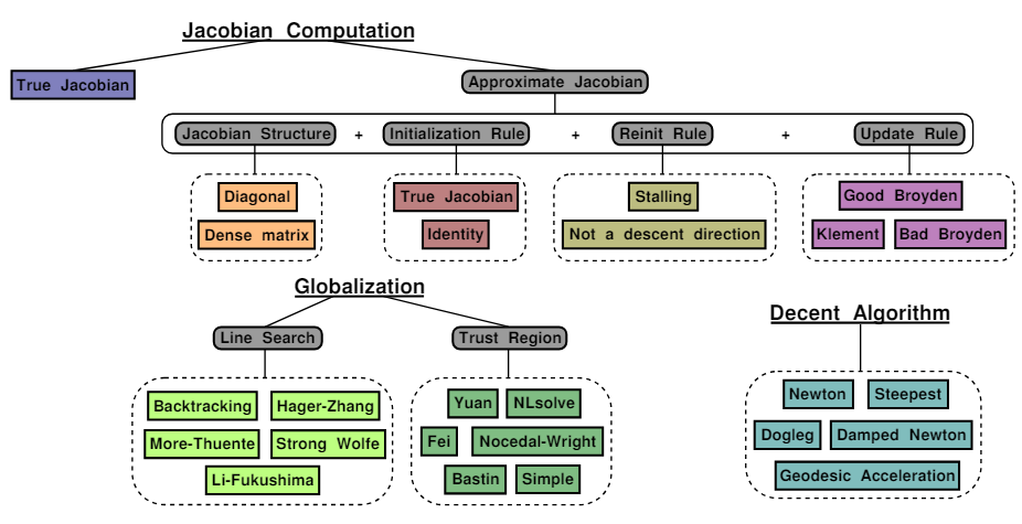
3.1. Composable Building Blocks
3.2. Smart PolyAlgortihm Defaults
3.3. Non-Allocating Static Algorithms inside GPU Kernels
3.4. Automatic Sparsity Exploitation
3.5. Generalized Jacobian-Free Nonlinear Solvers using Krylov Methods
4. Results and 4.1. Robustness on 23 Test Problems
4.2. Initializing the Doyle-Fuller-Newman (DFN) Battery Model
4.3. Large Ill-Conditioned Nonlinear Brusselator System
3. Special Capabilities
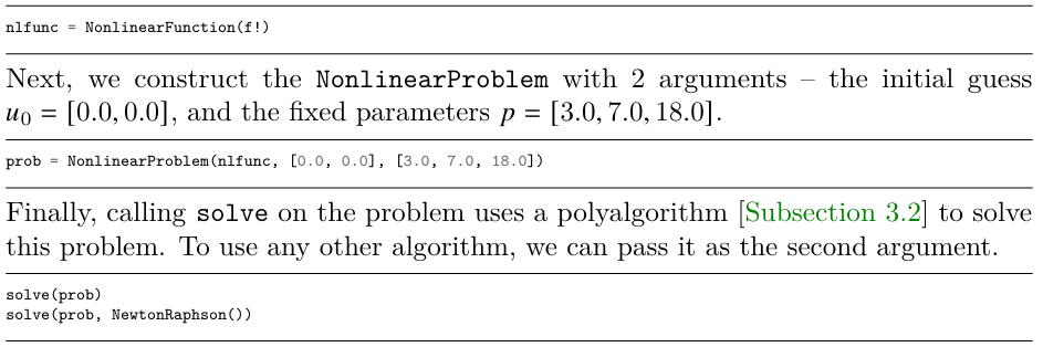
In the previous section, we provided an overview of solving nonlinear equations. Here, we will focus on specific capabilities of our package NonlinearSolve.jl. Let’s cover the typical workflow of using NonlinearSolve.jl. First, we define the nonlinear equations. We will use a mutating function to compute our residual value from 𝑢 and 𝑝 and store it in F.
\
\ In Julia, mutating function names are appended with a . ! as a convention. Next, we construct a NonlinearFunction – a wrapper over f! that can store additional information like user-defined Jacobian functions and sparsity patterns.
\
\
:::info This paper is available on arxiv under CC BY 4.0 DEED license.
:::
:::info Authors:
(1) AVIK PAL, CSAIL MIT, Cambridge, MA;
(2) FLEMMING HOLTORF;
(3) AXEL LARSSON;
(4) TORKEL LOMAN;
(5) UTKARSH;
(6) FRANK SCHÄFER;
(7) QINGYU QU;
(8) ALAN EDELMAN;
(9) CHRIS RACKAUCKAS, CSAIL MIT, Cambridge, MA.
:::
\
This content originally appeared on HackerNoon and was authored by Linearization Technology
Linearization Technology | Sciencx (2025-03-26T23:48:17+00:00) What Are the Special Capabilities of NonlinearSolve.jl?. Retrieved from https://www.scien.cx/2025/03/26/what-are-the-special-capabilities-of-nonlinearsolve-jl/
Please log in to upload a file.
There are no updates yet.
Click the Upload button above to add an update.