ZeroToGPT: A comprehensive guide to train Custom GPT from scratch on 7B tokens for free.

This content originally appeared on Level Up Coding - Medium and was authored by Umer Ateeq

TABLE OF CONTENT

1. Introduction
1.1 The Evolution from RNNs to Transformers
1.1.1 The Era of Recurrent Neural Networks
1.1.2 Fundamental Limitations of RNNs
1.1.3 The Transformer Revolution
1.1.4 The Breakthrough Paper
1.1.5 Core Architectural Innovation
1.1.6 Building the Complete Architecture

2. Dataset Importing
2.1 Input Embedding
2.2 Batch Loading
2.2.1 Configuration Setup
2.2.2 The get_batch Function Purpose
2.2.3 Memory-Mapped File Loading
2.2.4 Random Sampling Strategy
2.2.5 Input-Output Pair Creation
2.2.6 Data Type Conversion
2.2.7 Efficient GPU Transfer
2.2.8 Return Values

3. Positional Encoding

4. Attention
4.1 Step-by-Step Breakdown
4.1.1 Dot Product
4.1.2 Scale it
4.1.3 Apply Softmax
4.1.4 Multiply by V

5. Multi-Head Attention
5.1 Input and Output Dimensions (d_in, d_out)
5.2 Multiple Attention Heads (num_heads)
5.3 Linear Layers for Queries, Keys, and Values
5.4 Output Projection
5.5 Dropout Regularization
5.6 Causal Masking
5.7 Forward Pass (forward method)
5.8 Final Output

6. Layer-Normalization
6.1 What is LayerNorm?
6.2 Why Use LayerNorm?

7. Feed-Forward Block

8. Decoder Head
8.1 What Is a Decoder Block?
8.2 How It Works
8.2.1 Layer Normalization Before Attention
8.2.2 Causal Self-Attention
8.2.3 Residual Connection & Dropout (Post-Attention)
8.2.4 Second Layer Normalization
8.2.5 Feed-Forward Network (FFN)
8.2.6 Residual Connection & Dropout (Post-FFN)

9. GPT Block
9.1 Input Embedding and Positional Encoding
9.2 Shifted Output Embedding
9.3 Masked Multi-Head Attention
9.4 Add and Layer Normalization
9.5 Feed-Forward Neural Network
9.6 Second Add and Layer Normalization
9.7 Final Linear and Softmax Layer
9.8 Output Token Prediction
9.9 Token Embedding Layer
9.10 Positional Embedding Layer
9.11 Dropout on Input Embeddings
9.12 Transformer Block Stack
9.13 Final Normalization
9.14 Output Projection
9.15 Model Initialization
9.15.1 Model Configuration Setup
9.15.2 Random Seed Setting
9.15.3 Model Instantiation
9.15.4 Device Selection
9.15.5 Model Transfer to Device
9.15.6 Parameter Count Display
9.15.7 Device Confirmation

10.Training
10.1 Learning Rate Scheduler
10.1.1 Learning Rate Parameters Setup
10.1.2 Training Duration Configuration
10.1.3 Warmup Period Definition
10.1.4 Evaluation Frequency Setting
10.1.5 Batch Processing Parameters
10.1.6 Context Window Configuration
10.1.7 Gradient Accumulation Setup
10.1.8 Total Iteration Calculation
10.1.9 Optimizer Configuration
10.1.10 Warmup Scheduler Creation
10.1.11 Decay Scheduler Setup
10.1.12 Combined Scheduling Strategy
10.1.13 Regularization Through Weight Decay
10.1.14 Numerical Stability Considerations

10.2 Training Loop
10.2.1 Function Purpose and Parameters
10.2.2 Metric Tracking Setup
10.2.3 Mixed Precision Training Configuration
10.2.4 Gradient Scaler Initialization
10.2.5 Model Preparation
10.2.6 Outer Training Loop
10.2.7 Batch Processing Loop
10.2.8 Data Loading and Device Transfer
10.2.9 Forward Pass with Mixed Precision
10.2.10 Loss Normalization for Gradient Accumulation
10.2.11 Backward Pass with Gradient Scaling
10.2.12 Gradient Accumulation Logic
10.2.13 Gradient Clipping
10.2.14 Parameter Updates
10.2.15 Learning Rate Scheduling
10.2.16 Gradient Reset
10.2.17 Token Counting and Step Tracking
10.2.18 Evaluation Checkpoints
10.2.19 Loss Computation and Storage
10.2.20 Progress Reporting
10.2.21 Text Generation Sampling
10.2.22 Return Values

11.Inference
11.1 Tokenizer Initialization
11.2 Core Text Generation Function
11.2.1 Function Purpose
11.2.2 Context Window Management
11.2.3 Model Prediction Process
11.2.4 Last Token Focus
11.2.5 Probability Conversion
11.2.6 Token Selection Strategy
11.2.7 Sequence Extension
11.3 Text to Token Conversion Function
11.3.1 Encoding Process
11.3.2 Batch Dimension Addition
11.4 Token to Text Conversion Function
11.4.1 Decoding Process
11.4.2 Batch Dimension Removal
11.5 Sample Generation and Display Function
11.5.1 Model State Management
11.5.2 Context Size Detection
11.5.3 Input Preparation
11.5.4 Generation Execution
11.5.5 Output Formatting
11.5.6 Model State Restoration
11.6 Example Usage Section
11.6.1 Context Definition
11.6.2 Generation Parameters
11.6.3 Device Management
11.6.4 Output Display
11.7 Key Generation Concepts
11.7.1 Autoregressive Nature
11.7.2 Context Sliding Window
11.7.3 Deterministic Selection

12.Evaluation and Results
12.1 Loss Calculation Functions Explanation
12.1.1 Function Purpose
12.1.2 Input Data Preparation
12.1.3 Model Forward Pass
12.1.4 Tensor Reshaping for Loss Computation
12.1.5 Cross-Entropy Loss Calculation
12.2 Data Loader Loss Calculation Function
12.2.1 Function Overview
12.2.2 Empty Data Loader Handling
12.2.3 Batch Count Determination
12.2.4 Batch Count Safety Check
12.2.5 Iterative Loss Accumulation
12.2.6 Early Termination Logic
12.2.7 Average Loss Computation
12.3 Model Evaluation Function
12.3.1 Evaluation Setup
12.3.2 Training Data Evaluation
12.3.3 Validation Data Evaluation
12.3.4 Gradient Computation Disabled
12.3.5 Model Mode Restoration
12.3.6 Return Values

13.RESULTS

1) Introduction:

In recent years, large language models (LLMs) have reshaped the world of artificial intelligence, enabling machines to generate coherent, creative, and often human-like responses across a wide range of tasks. This transformation became widely recognized with the public release of ChatGPT in late November 2022, marking a pivotal moment in AI adoption. The capabilities of ChatGPT astonished both the general public and the scientific community — setting off what many now refer to as the “LLM revolution.”

Inspired by this, we sought to move beyond just using pretrained models. While many rely on open-sourced weights from models like GPT-2 or GPT-3, few attempt to train such models from scratch. This is largely due to two major challenges:

1. High hardware requirements, and

2. Significant technical complexity.

In this project, we embraced both challenges and undertook the ambitious task of building a large language model from scratch. Our goal was not just to replicate results but to understand the inner workings of these architectures through hands-on implementation, experimentation, and iteration.

Our journey began with the foundational paper “Attention is All You Need” (Vaswani et al., 2017), which introduced the attention mechanism and the transformer architecture composed of encoder-decoder blocks. From there, we transitioned toward the GPT-2 paper by OpenAI, which simplified the architecture by removing the encoder and focusing solely on a decoder-only model.

Based on this, we designed and trained our own transformer model consisting of 12 decoder layers and 8 attention heads. This project served as both a practical implementation and a deep exploration into the effectiveness of attention mechanisms at scale.

1.1 The Evolution from RNNs to Transformers

1.1.1 The Era of Recurrent Neural Networks

Before the transformer revolution, Recurrent Neural Networks (RNNs) were the dominant architecture for processing sequential data. These networks processed information step by step, maintaining hidden states that carried information from previous time steps to current ones.

1.1.2 Fundamental Limitations of RNNs

Despite their widespread adoption, RNNs suffered from several critical limitations that hindered their effectiveness:

Gradient Flow Problems: RNNs were plagued by exploding and vanishing gradient issues, making it difficult to train deep networks effectively and learn long-range dependencies.

Sequential Processing Bottleneck: The inherent sequential nature of RNNs created a computational bottleneck. Each time step had to wait for the previous computation to complete, preventing parallel processing and significantly slowing down training and inference.

Long Sequence Degradation: As sequence length increased, RNNs struggled to maintain relevant information from distant past states, leading to poor performance on tasks requiring long-term memory.

1.1.3 The Transformer Revolution

1.1.4 The Breakthrough Paper

In 2017, the groundbreaking paper “Attention Is All You Need” introduced the Transformer architecture, fundamentally changing the landscape of natural language processing and sequence modeling. This innovation eliminated the need for recurrent connections entirely.

1.1.5 Core Architectural Innovation

The original Transformer architecture consists of two primary components working in tandem:

Encoder Block: Processes the input sequence and creates rich contextual representations of the data.

Decoder Block: Generates output sequences while attending to both the input representations and previously generated tokens.

1.1.6 Building the Complete Architecture

Understanding the Transformer requires examining its construction from the ground up. We begin with the fundamental layers that comprise each block, then explore how these layers combine to form the encoder and decoder components, and finally examine how these blocks work together to create the complete Transformer architecture.

This hierarchical approach — from individual layers to complete blocks to the full architecture — provides a comprehensive understanding of how Transformers revolutionized sequence processing and paved the way for modern language models like GPT.

Lets focus on building each and every block step by step and then will merge them.

2) Dataset importing:

!pip install --upgrade datasets huggingface_hub fsspec
from datasets import load_dataset

text_data = load_dataset("roneneldan/TinyStories", cache_dir="/content/hf_datasets_cache")
print(text_data)

using this below code we have imported our Dataset from Hugging Face which is approx 0.5B tokens into our RAM by using text_data variable.

our output text_data is this:

DatasetDict({
    train: Dataset({
        features: ['text'],
        num_rows: 2119719
    })
    validation: Dataset({
        features: ['text'],
        num_rows: 21990
    })
})

now, its time to convert it into tokens which we will do using a tokenizer by OpenAI.

2.1.1 Input Embedding:

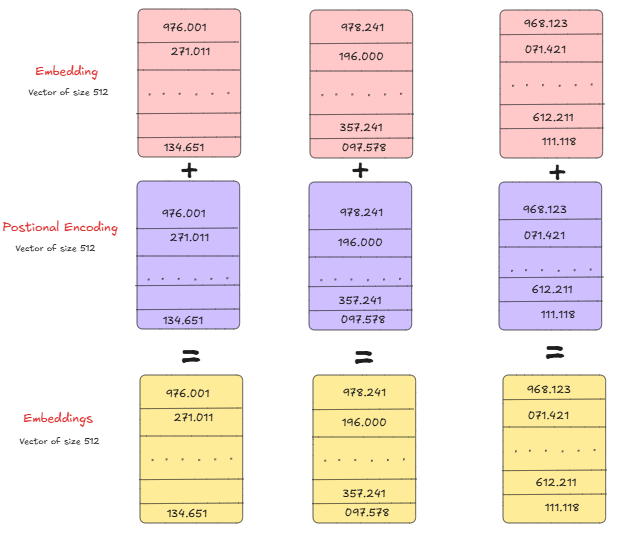
In natural language processing with transformers, raw text needs to be converted into numerical representations that models can understand. This is done using embeddings, where each token is mapped to a high-dimensional vector capturing semantic meaning.

!pip install tiktoken
import tiktoken
enc = tiktoken.get_encoding("gpt2")

def tokenizing_func(example):
    ids = enc.encode_ordinary(example['text']) # encode_ordinary ignores any special tokens
    out = {'ids': ids, 'len': len(ids)}
    return out

now, we will see this function in action:

tokenized_data = text_data.map(
    tokenizing_func,
    remove_columns=['text'],# this will drop "text" column from tokenized_data.
    num_proc=8 # Enables multiprocessing to 8 CPUs
    )

We are using .map() from the Hugging Face Datasets library — one of its most powerful and flexible functions for preprocessing.

Applies a function (tokenizing_func here) to each example (or batch of examples) in our dataset. It returns a new dataset with transformed outputs.

NOW, we will do PRE-TOKENIZATION and next the below block of code is converting our tokenized dataset into a single, flat binary file (.bin) that can be memory-mapped and used for efficient training, especially for transformer models like GPT.

import os
import numpy as np
from tqdm.auto import tqdm

if not os.path.exists("train.bin"):
    tokenized = text_data.map(
        tokenizing_func,
        remove_columns=['text'],
        desc="tokenizing the splits",
        num_proc=8,
        )
    # concatenate all the ids in each dataset into one large file we can use for training
    for split, dset in tokenized.items():
        arr_len = np.sum(dset['len'], dtype=np.uint64)
        filename = f'{split}.bin'
        dtype = np.uint16 # (can do since enc.max_token_value == 50256 is < 2**16)
        arr = np.memmap(filename, dtype=dtype, mode='w+', shape=(arr_len,))
        total_batches = 1024

        idx = 0
        for batch_idx in tqdm(range(total_batches), desc=f'writing {filename}'):
            # Batch together samples for faster write
            batch = dset.shard(num_shards=total_batches, index=batch_idx, contiguous=True).with_format('numpy')
            arr_batch = np.concatenate(batch['ids'])
            # Write into mmap
            arr[idx : idx + len(arr_batch)] = arr_batch
            idx += len(arr_batch)
        arr.flush()

for even more bigger datasets we enable streaming and for that we use a little different strategy:

2.2 Batch Loading:

2.2.1 Configuration Setup

The code begins by extracting key parameters from the GPT configuration dictionary. The block_size represents the maximum sequence length (context window) that the model can process at once, while batch_size determines how many training examples are processed simultaneously during each training step.

2.2.2 The get_batch Function Purpose

This function is responsible for loading and preparing training data batches for the GPT model. It handles the critical task of creating input-output pairs from the tokenized text data, where the model learns to predict the next token given a sequence of previous tokens.

2.2.3 Memory-Mapped File Loading

The function uses NumPy’s memory mapping feature to efficiently access large datasets without loading everything into RAM. Based on the split parameter, it loads either training data from train.bin or validation data from validation.bin. These binary files contain tokenized text data stored as 16-bit unsigned integers.

The memory mapping is recreated for each batch to prevent memory leaks, following best practices for handling large datasets.

2.2.4 Random Sampling Strategy

The code generates random starting positions within the dataset using torch.randint. It creates batch_size number of random indices, ensuring each starting position allows for a complete sequence of block_size tokens plus one additional token for the target.

2.2.5 Input-Output Pair Creation

For each random starting position, the function creates two sequences:

Input sequence (x): Contains tokens from position i to i + block_size, representing the context the model uses to make predictions.

Target sequence (y): Contains tokens from position i + 1 to i + 1 + block_size, representing the ground truth next tokens the model should predict.

This creates the classic language modeling setup where each token in the input corresponds to predicting the next token in the target sequence.

2.2.6 Data Type Conversion

The data is converted from NumPy arrays to PyTorch tensors, with dtype conversion from uint16 to int64 to match PyTorch’s expected integer format for token indices.

2.2.7 Efficient GPU Transfer

The function includes optimized GPU memory transfer logic. When CUDA is available, it uses memory pinning (pin_memory()) combined with asynchronous transfer (non_blocking=True) to move data to GPU more efficiently. This technique allows the CPU to continue processing while the GPU transfer happens in the background.

When CUDA is not available, it simply moves the tensors to the specified device (typically CPU).

2.2.8 Return Values

The function returns a tuple containing the input sequences (x) and their corresponding target sequences (y), both properly formatted as PyTorch tensors on the appropriate computing device, ready for training or evaluation.

block_size  = GPT_CONFIG_124M['context_length']
batch_size = GPT_CONFIG_124M['batch_size']
# Some functions from https://github.com/karpathy/nanoGPT/blob/master/train.py with slight modifications
def get_batch(split):
    # We recreate np.memmap every batch to avoid a memory leak, as per
    # https://stackoverflow.com/questions/45132940/numpy-memmap-memory-usage-want-to-iterate-once/61472122#61472122
    if split == 'train':
        data = np.memmap('train.bin', dtype=np.uint16, mode='r')
    else: # '/content/drive/MyDrive/tokenized/validation.bin',
        data = np.memmap('validation.bin', dtype=np.uint16, mode='r')
    ix = torch.randint(len(data) - block_size, (batch_size,))
    x = torch.stack([torch.from_numpy((data[i:i+block_size]).astype(np.int64)) for i in ix])
    y = torch.stack([torch.from_numpy((data[i+1:i+1+block_size]).astype(np.int64)) for i in ix])
    if torch.cuda.is_available() == True:
        # pin arrays x,y, which allows us to move them to GPU asynchronously (non_blocking=True)
        x, y = x.pin_memory().to(device, non_blocking=True), y.pin_memory().to(device, non_blocking=True)
    else:
        x, y = x.to(device), y.to(device)
    return x, y

3) Positional encoding:

we have a slight problem with the attention mechanism, it has no internal mechanism to keep track of the position of every word/token. So, that’s why we have to manually provide it with the position of each token and we do it by using positional encoding with the formula written in the image above.

We can visualize it below:

coding explanation is this:

class PositionalEncoding(nn.Module):
    def __init__(self, d_model, max_seq_length):
        super(PositionalEncoding, self).__init__()

        pe = torch.zeros(max_seq_length, d_model)
        position = torch.arange(0, max_seq_length, dtype=torch.float).unsqueeze(1)
        div_term = torch.exp(torch.arange(0, d_model, 2).float() * -(math.log(10000.0) / d_model))

        pe[:, 0::2] = torch.sin(position * div_term)
        pe[:, 1::2] = torch.cos(position * div_term)

        self.register_buffer('pe', pe.unsqueeze(0))

    def forward(self, x):
        return x + self.pe[:, :x.size(1)]

Using this we encode the position of a word in a sentence.

4) Attention:

Attention is an efficient way to compute a context-dependent correlation matrix between elements (like words or tokens) in a sequence.

Q, K, V are matrices and all are equal to x(input/tokenzed data)

4.1) Step-by-Step Breakdown

4.1.1 Dot Product:

You compare your Query with every Key using a dot product, which gives you a similarity score for each pair.

High dot product → high similarity
Low dot product → less relevant

This creates a matrix of scores, where each token knows how much it should pay attention to others.

4.1.2 Scale it:

The dot product can get large if your vectors are long. This can make the softmax too sharp (it picks one word with almost 100% weight).

To fix that, we divide by square root of dk

4.1.3 Apply Softmax:

Now we apply softmax, which turns these scores into a probability distribution.

Each row in the matrix becomes a list of weights.
The weights add up to 1.
A higher weight means more attention is paid to that token.

4.1.4 Multiply by V

Now that you have weights (from softmax), you multiply them with the Values (V) and sum them up.

That gives a new vector — a combination of other token values — based on how relevant they are to your Query.

def _scaled_dot_attention(self, q, k, v, mask=None):
        # q, k, v: (b, num_heads, seq_len, head_dim)
        attn_scores = q @ k.transpose(-2, -1)  # (b, num_heads, t_q, t_k)
        attn_scores /= self.head_dim ** 0.5
       
        attn_weights = torch.softmax(attn_scores, dim=-1)
        attn_weights = self.dropout(attn_weights)
        return attn_weights @ v  # (b, num_heads, seq_len, head_dim)

5) Multi-Head Attention:

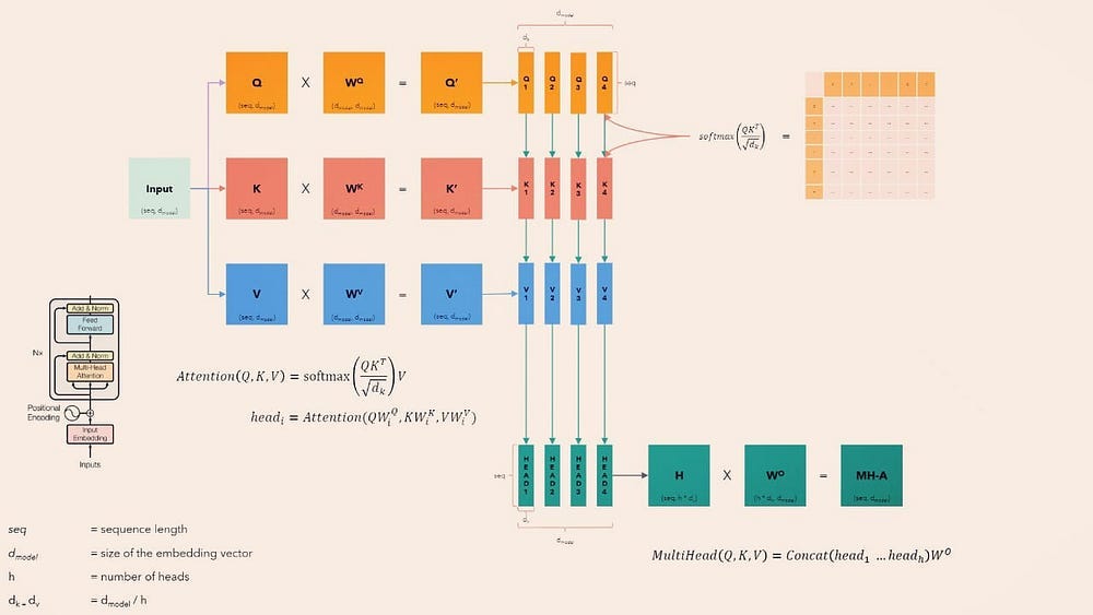
The MultiHeadAttention module is a fundamental building block of the Transformer architecture. Its main job is to enable the model to focus on different parts of the input sequence simultaneously — capturing relationships and dependencies between tokens (words or subwords) regardless of their position.🔧 Initialization (__init__ method)

5.1 Input and Output Dimensions (d_in, d_out)

The model receives input embeddings of size d_in and produces output embeddings of size d_out. These embeddings represent tokens in high-dimensional space.

5.2 Multiple Attention Heads (num_heads)

The total output dimension (d_out) is divided evenly across multiple attention heads. Each head focuses on a different “subspace” of the input, allowing the model to capture a richer variety of relationships. For example, one head might focus on syntactic relationships, while another might capture semantic similarity.

5.3 Linear Layers for Queries, Keys, and Values

Three separate linear transformations project the input into:

Queries (Q): what a token is looking for.

Keys (K): what a token offers.

Values (V): The actual content/information of the token.

These projections are computed independently for each attention head.

5.4 Output Projection

After each attention head processes its data, their outputs are concatenated and passed through another linear layer to mix them together.

5.5 Dropout Regularization

Dropout is applied to the attention weights to reduce overfitting during training.

5.6 Causal Masking

A triangular mask prevents a token from attending to future tokens. This is crucial for autoregressive models (like GPT), where the model should only use past and present information when predicting the next token.

5.7 Forward Pass (forward method)

Input Shape Extraction
The input tensor x has shape (batch_size, num_tokens, d_in). This represents a batch of token sequences.

Linear Projections to Q, K, V
The input is passed through the three linear layers to obtain queries, keys, and values of shape (batch_size, num_tokens, d_out).

Reshape for Multi-Head Processing
These tensors are reshaped into multiple heads:

New shape: (batch_size, num_heads, num_tokens, head_dim)

This allows each attention head to operate independently on a different portion of the embedding.

Compute Scaled Dot-Product Attention
Each head calculates attention scores as a dot product between queries and keys. These scores are scaled by the square root of the dimensionality for numerical stability.

Apply Causal Mask
A triangular mask is applied to the attention scores to block attention to future tokens. This ensures that the model only uses available (past and current) context during training or generation.

Softmax Normalization and Dropout
The masked attention scores are passed through a softmax to get attention weights — essentially telling the model “how much to attend” to each token. Dropout is then applied for regularization.

Compute Contextualized Values
The attention weights are used to compute a weighted average of the value vectors. This yields a new, context-aware representation for each token.

Concatenate and Project
The outputs from all heads are combined and passed through the output projection layer to match the expected dimensionality (d_out).

5.8 Final Output

The final tensor has the same shape as the input:
(batch_size, num_tokens, d_out),
but now each token has been transformed using contextual information from surrounding tokens — with multiple heads capturing different perspectives.

This is the power of self-attention: it allows each word to be dynamically informed by others, depending on learned relevance, enabling the Transformer to model long-range dependencies effectively.Compute Contextualized Values
The attention weights are used to compute a weighted average of the value vectors. This yields a new, context-aware representation for each token.

Concatenate and Project
The outputs from all heads are combined and passed through the output projection layer to match the expected dimensionality (d_out)

5.8 FINAL OUTPUT:

import torch
import torch.nn as nn

class MultiHeadAttention(nn.Module):
    def __init__(self, d_in, d_out, context_length, dropout, num_heads, qkv_bias=False):
        super().__init__()
        assert d_out % num_heads == 0, "d_out must be divisible by num_heads"
        
        self.d_out = d_out
        self.num_heads = num_heads
        self.head_dim = d_out // num_heads
        self.context_length = context_length
        
        # Linear projections for Q, K, V
        self.W_q = nn.Linear(d_in, d_out, bias=qkv_bias)
        self.W_k = nn.Linear(d_in, d_out, bias=qkv_bias)
        self.W_v = nn.Linear(d_in, d_out, bias=qkv_bias)
        
        # Output projection after concatenation of all heads
        self.out_proj = nn.Linear(d_out, d_out)
        self.dropout = nn.Dropout(dropout)
        
        # Causal mask using Code 2's logic (True = masked position)
        self.register_buffer("causal_mask", torch.triu(torch.ones(context_length, context_length), diagonal=1).bool())
    
    def _split_heads(self, x):
        # x: (b, seq_len, d_out) → (b, num_heads, seq_len, head_dim)
        b, t, _ = x.size()
        return x.view(b, t, self.num_heads, self.head_dim).transpose(1, 2)
    
    def _combine_heads(self, x):
        # x: (b, num_heads, seq_len, head_dim) → (b, seq_len, d_out)
        b, nh, t, hd = x.size()
        return x.transpose(1, 2).contiguous().view(b, t, nh * hd)
    
    def _scaled_dot_attention(self, q, k, v, mask=None):
        # q, k, v: (b, num_heads, seq_len, head_dim)
        attn_scores = q @ k.transpose(-2, -1)  # (b, num_heads, t_q, t_k)
        attn_scores /= self.head_dim ** 0.5
        
        # Apply mask using Code 2's logic (True = mask position)
        if mask is not None:
            attn_scores = attn_scores.masked_fill(mask, float('-inf'))
        
        attn_weights = torch.softmax(attn_scores, dim=-1)
        attn_weights = self.dropout(attn_weights)
        return attn_weights @ v  # (b, num_heads, seq_len, head_dim)
    
    def forward(self, x=None, q=None, k=None, v=None, mask=None):
        # If q/k/v not provided, default to self-attention using x
        if q is None and k is None and v is None:
            q = k = v = x
        elif q is None or k is None or v is None:
            raise ValueError("Either provide all of q/k/v or none.")
        
        b, t, _ = q.size()
        
        # Apply linear projections
        q_proj = self.W_q(q)
        k_proj = self.W_k(k)
        v_proj = self.W_v(v)
        
        # Split heads
        q_split = self._split_heads(q_proj)
        k_split = self._split_heads(k_proj)
        v_split = self._split_heads(v_proj)
        
        # Apply causal mask using Code 2's logic if none is provided
        if mask is None and x is not None:
            # Create causal mask where True = masked position
            mask = self.causal_mask[:t, :t].unsqueeze(0).unsqueeze(0).to(q.device)
        
        # Scaled dot-product attention
        context = self._scaled_dot_attention(q_split, k_split, v_split, mask)
        
        # Combine heads and apply output projection
        context = self._combine_heads(context)
        return self.out_proj(context)

6) Layer-Normalization:

6.1 What is LayerNorm?

Layer Normalization (LayerNorm) is a technique used in deep learning to stabilize and accelerate training by normalizing the inputs to each layer. Unlike BatchNorm, which normalizes across the batch dimension, LayerNorm normalizes across the features of each individual data point.

It was introduced in the paper:
📄 Layer Normalization (Ba et al., 2016)

6.2 Why Use LayerNorm?

When training deep networks:

Inputs to layers can shift in distribution, known as internal covariate shift.
This makes optimization harder and slows down convergence.

LayerNorm combats this by ensuring:

The mean is zero and the variance is one across the features for every token or sample.
It helps gradients flow better through the network.
It enables faster and more stable training, especially in transformers, where it’s a standard component.

Layer Normalization is a technique used to stabilize and speed up training by normalizing the values in a layer — so they have mean = 0 and variance = 1 — across the features of a single example.

class LayerNorm(nn.Module):
    def __init__(self, emb_dim):
        super().__init__()
        self.eps = 1e-5
        self.scale = nn.Parameter(torch.ones(emb_dim))
        self.shift = nn.Parameter(torch.zeros(emb_dim))

    def forward(self, x):
        mean = x.mean(dim=-1, keepdim=True)
        var = x.var(dim=-1, keepdim=True, unbiased=False)
        norm_x = (x - mean) / torch.sqrt(var + self.eps)
        return self.scale * norm_x + self.shift

7) Feed-Forward Block:

In Transformer architectures, the Feed-Forward Network (FFN) is applied independently to each token, after the attention mechanism. It introduces non-linearity and depth, helping the model learn richer representations.

This FeedForward module implements that FFN block.

class FeedForward(nn.Module):
    def __init__(self, cfg):
        super().__init__()
        self.layers = nn.Sequential(
            nn.Linear(cfg["emb_dim"], 4 * cfg["emb_dim"]),
            nn.ReLU(),
            nn.Linear(4 * cfg["emb_dim"], cfg["emb_dim"]),
        )

    def forward(self, x):
        return self.layers(x)

Input Dim: cfg["emb_dim"]

The input is a vector of size emb_dim (i.e., the embedding dimension for each token).

Hidden Layer: 4 * emb_dim

The first linear layer expands the size from emb_dim to 4 * emb_dim.
This expansion gives the model more capacity to learn complex transformations.

Activation Function: ReLU()

Introduces non-linearity, which allows the model to learn non-trivial functions.

Helps break symmetry and adds expressive power.

Output Layer: Back to emb_dim

The second linear layer compresses the vector back to the original emb_dim.

This pattern (Linear -> ReLU -> Linear) is very common in transformers and is often referred to as a position-wise feed-forward network, because it operates on each token vector individually (not across time or batch).

8) Decoder head:

8.1 What Is a Decoder Block?

A Decoder Block is a key component in decoder-only Transformer models like GPT. It is designed to process a sequence of token embeddings and gradually build a deeper understanding of the input context by repeatedly applying self-attention, normalization, and feed-forward transformations.

8.2 How It Works

The Decoder Block performs the following operations in sequence:

8.2.1 Layer Normalization Before Attention:
The input is first normalized using LayerNorm, which stabilizes the learning process and ensures consistent scaling of input features.

8.2.2 Causal Self-Attention:
The normalized input passes through a multi-head self-attention mechanism. This allows each token to selectively focus on previous tokens in the sequence — learning how they relate, while maintaining causality (i.e., not looking ahead).

8.2.3 Residual Connection & Dropout (Post-Attention):
The output of the attention mechanism is regularized using dropout and then added back to the original input (via a residual connection). This skip connection helps with gradient flow and preserves useful features from earlier layers.

8.2.4 Second Layer Normalization:
Another LayerNorm is applied, this time before the next component — the feed-forward network.

8.2.5 Feed-Forward Network (FFN):
This is a simple neural network applied independently to each token. It expands the embedding dimension temporarily, applies a non-linearity (like ReLU), and then projects it back. This step adds non-linear transformations and allows the model to better represent complex patterns.

8.2.6 Residual Connection & Dropout (Post-FFN):
Again, the FFN output is passed through dropout and added to its input using a residual connection, just like in the attention part.

class DecoderBlock(nn.Module):
    def __init__(self, cfg):
        super().__init__()
        self.att = MultiHeadAttention(
            d_in=cfg["emb_dim"],
            d_out=cfg["emb_dim"],
            context_length=cfg["context_length"],
            num_heads=cfg["n_heads"],
            dropout=cfg["drop_rate"],
            qkv_bias=cfg["qkv_bias"])
        self.ff = FeedForward(cfg)
        self.norm1 = LayerNorm(cfg["emb_dim"])
        self.norm2 = LayerNorm(cfg["emb_dim"])
        self.drop_shortcut = nn.Dropout(cfg["drop_rate"])

    def forward(self, x):
        # Shortcut connection for attention block
        shortcut = x
        x = self.norm1(x)
        x = self.att(x)  # Shape [batch_size, num_tokens, emb_size]
        x = self.drop_shortcut(x)
        x = x + shortcut  # Add the original input back

        # Shortcut connection for feed forward block
        shortcut = x
        x = self.norm2(x)
        x = self.ff(x)
        x = self.drop_shortcut(x)
        x = x + shortcut  # Add the original input back

        return x

9) GPT-BLOCK:

9.1 Input Embedding and Positional Encoding

The input tokens are first converted into vector representations using an embedding layer. Since the transformer doesn’t inherently know the order of tokens, positional encodings are added to inject information about the position of each token in the sequence. This combined representation serves as the input to the decoder.

9.2 Shifted Output Embedding

The expected output sequence (during training) is also embedded and shifted one position to the right. This is done so the model predicts the next token without seeing it directly, ensuring autoregressive behavior.

9.3 Masked Multi-Head Attention

This layer allows each token to attend to earlier tokens in the sequence. A mask is applied so that a token cannot see future tokens — only the current and previous ones — preserving the left-to-right generation flow.

9.4 Add and Layer Normalization

The output of the masked attention layer is added back to the original input of the layer (residual connection), and then normalized. This helps stabilize and speed up training.

9.5 Feed Forward Neural Network

A small neural network processes each position in the sequence independently. It usually has two linear layers with a non-linearity in between to increase the model’s expressive power.

9.6 Second Add and Layer Normalization

The output of the feed-forward network is again added back to its input and normalized, following the same residual and normalization pattern.

9.7 Final Linear and Softmax Layer

After all the decoder blocks, a final linear layer maps the processed token representations to a vector the size of the vocabulary. A softmax is then applied to get a probability distribution over all possible next tokens.

9.8 Output Token Prediction

The model uses the probabilities from the softmax layer to predict the most likely next token in the sequence, enabling language generation.

here we have coded it:

class GPTModel(nn.Module):
    def __init__(self, cfg):
        super().__init__()
        self.tok_emb = nn.Embedding(cfg["vocab_size"], cfg["emb_dim"])
        self.pos_emb = nn.Embedding(cfg["context_length"], cfg["emb_dim"])
        self.drop_emb = nn.Dropout(cfg["drop_rate"])

        self.trf_blocks = nn.Sequential(
            *[TransformerBlock(cfg) for _ in range(cfg["n_layers"])])

        self.final_norm = LayerNorm(cfg["emb_dim"])
        self.out_head = nn.Linear(
            cfg["emb_dim"], cfg["vocab_size"], bias=False
        )

    def forward(self, in_idx):
        batch_size, seq_len = in_idx.shape
        tok_embeds = self.tok_emb(in_idx)
        pos_embeds = self.pos_emb(torch.arange(seq_len, device=in_idx.device))
        x = tok_embeds + pos_embeds  # Shape [batch_size, num_tokens, emb_size]
        x = self.drop_emb(x)
        x = self.trf_blocks(x)
        x = self.final_norm(x)
        logits = self.out_head(x)
        return logits

9.9 Token Embedding Layer

The model begins by converting each input token (represented by an integer ID) into a dense vector using an embedding layer. This turns raw token IDs into meaningful representations that the model can work with.

9.10 Positional Embedding Layer

Since the Transformer does not inherently understand the order of tokens, a separate positional embedding is used. This adds information about the position of each token in the sequence, helping the model to distinguish between, for example, a word at the beginning of the sentence and the same word at the end.

9.11 Dropout on Input Embeddings

After combining token embeddings and positional embeddings, a dropout layer is applied. This randomly disables a small portion of the information during training to prevent overfitting and make the model more robust.

9.12 Transformer Block Stack

The core of the model is a stack of Transformer blocks. Each block contains self-attention mechanisms and feedforward layers that allow the model to learn complex relationships between tokens. These blocks are applied sequentially, refining the representations at each step.

9.13 Final Normalization

Once the data has passed through all the Transformer blocks, it goes through one last layer normalization. This helps stabilize the output and ensures that the final values are well-behaved for the next stage.

9.14 Output

The final representation is passed through a linear layer that maps it to a vector the size of the vocabulary. This gives the model’s prediction scores for the next token in the sequence at each position.

The model returns the raw scores, called logits, for each token position. These can be used to compute probabilities over the vocabulary and select the most likely next token during text generation.

9.15 Model Initialization:

9.15.1 Model Configuration Setup

The code defines a configuration dictionary that specifies how the GPT model should be built. This includes settings for the model’s size, structure, and training parameters like vocabulary size, embedding dimensions, and number of layers.

9.15.2 Random Seed Setting

A random seed is set to ensure reproducible results. This means every time you run the code, you’ll get the same random initialization of the model weights.

9.15.3 Model Instantiation

The GPT model is created using the configuration settings defined earlier. This builds the entire neural network architecture with all its layers and components.

9.15.4 Device Selection

The code checks if a GPU is available on the system. If CUDA-compatible GPU hardware is found, it will use that for faster computation. Otherwise, it falls back to using the CPU.

9.15.5 Model Transfer to Device

The model is moved to the selected computing device (either GPU or CPU) so all calculations will happen on the appropriate hardware.

9.15.6 Parameter Count Display

The total number of trainable parameters in the model is calculated and displayed in millions. This gives you an idea of the model’s size and complexity.

9.15.7 Device Confirmation

The code prints which device (CPU or GPU) is actually being used for computation, confirming the hardware setup.

GPT_CONFIG_124M = {
    "num_workers": 0, # usually 2-4 is safer! # This controls how many subprocesses PyTorch uses to load the data in parallel.
    "batch_size":256, # Llama 2 7B was trained with a batch size of 1024
    "context_length": 1024, # for 50% data overlap!
    "Stride":1024,
    "vocab_size": 50257,   # Vocabulary size
    "emb_dim": 1024,        # Embedding dimension
    "n_heads": 12,         # Number of attention heads
    "n_layers": 12,        # Number of layers
    "drop_rate": 0.1,      # Dropout rate
    "qkv_bias": False      # Query-key-value bias
}

torch.manual_seed(123)

model = GPTModel(GPT_CONFIG_124M)
device = torch.device("cuda" if torch.cuda.is_available() else "cpu")
model.to(device)

print(sum(p.numel() for p in model.parameters()) / 1e6, 'M parameters')
print(device)

10) TRAINING:

10.1 Learning Rate Scheduler:

10.1.1 Learning Rate Parameters Setup

The configuration establishes the learning rate boundaries for training. A higher initial learning rate allows for faster initial learning, while a lower minimum learning rate ensures stable convergence during the final stages of training.

10.1.2 Training Duration Configuration

The total training duration is defined through the number of epochs, which determines how many complete passes through the dataset the model will make during training.

10.1.3 Warmup Period Definition

A warmup period is configured to gradually increase the learning rate from zero to the maximum value over a specified number of steps. This prevents unstable training that can occur when starting with high learning rates.

10.1.4 Evaluation Frequency Setting

The evaluation frequency determines how often the model’s performance is assessed on validation data during training. More frequent evaluation provides better monitoring but increases computational overhead.

10.1.5 Batch Processing Parameters

The batch size controls how many training examples are processed simultaneously, affecting both memory usage and gradient estimation quality. Larger batches generally provide more stable gradient estimates.

10.1.6 Context Window Configuration

The block size defines the maximum sequence length the model can process at once, directly impacting the model’s ability to capture long-range dependencies in the text.

10.1.7 Gradient Accumulation Setup

Gradient accumulation allows for effective larger batch sizes by accumulating gradients across multiple smaller batches before updating model parameters. This technique helps when memory constraints prevent using large batches directly.

10.1.8 Total Iteration Calculation

The maximum number of training iterations is computed by multiplying the number of batches per epoch by the total number of epochs, providing the complete training schedule.

10.1.9 Optimizer Configuration

The AdamW optimizer is configured with specific parameters including momentum terms, weight decay for regularization, and numerical stability settings. The beta values control the momentum behavior, while weight decay helps prevent overfitting.

10.1.10 Warmup Scheduler Creation

A linear warmup scheduler is created to gradually increase the learning rate from zero to the maximum value over the specified warmup period. This helps stabilize early training dynamics.

10.1.11 Decay Scheduler Setup

A cosine annealing scheduler is configured to smoothly decrease the learning rate from the maximum value to the minimum value over the remaining training iterations. This schedule often leads to better final model performance.

10.1.12 Combined Scheduling Strategy

The warmup and decay schedulers are combined using a sequential scheduler that automatically switches from warmup to decay at the specified milestone. This creates a complete learning rate schedule that starts with gradual increase followed by smooth decay.

10.1.13 Regularization Through Weight Decay

Weight decay is incorporated as a regularization technique that prevents the model from overfitting by penalizing large parameter values. This helps the model generalize better to unseen data.

10.1.14 Numerical Stability Considerations

The epsilon parameter in the optimizer provides numerical stability by preventing division by very small numbers during the optimization process, which is particularly important when using mixed precision training.

# Training Hyperparameters
batch_size = 32
block_size = 128
learning_rate = 5e-4
min_lr = 1e-4
warmup_steps = 1000
num_epochs = 20
max_iters = GPT_CONFIG_124M['num_batches_per_epoch'] * num_epochs

# Optimizer
optimizer = torch.optim.AdamW(model.parameters(),lr=learning_rate,
betas=(0.9, 0.95), weight_decay=0.1, eps=1e-9 )

# Learning Rate Scheduler: Warmup + Cosine Decay
from torch.optim.lr_scheduler import LinearLR, SequentialLR, CosineAnnealingLR

scheduler = SequentialLR(
    optimizer,
    schedulers=[
       LinearLR(optimizer, total_iters=warmup_steps),
       CosineAnnealingLR(optimizer,T_max=max_iters-warmup_steps,eta_min=min_lr) 
            ],
        milestones=[warmup_steps] )

10.2 TRAINING LOOP:

10.2.1 Function Purpose and Parameters

This function implements a comprehensive training loop for GPT models with advanced optimization techniques. It accepts the model, optimizer, learning rate scheduler, and various training parameters including the number of epochs, evaluation frequency, and gradient accumulation settings.

10.2.2 Metric Tracking Setup

The function initializes empty lists to track training progress including training losses, validation losses, and the number of tokens processed. It also sets up counters for tokens seen and global training steps.

10.2.3 Mixed Precision Training Configuration

Mixed precision training is enabled using PyTorch’s automatic mixed precision capabilities. This technique uses lower precision floating point numbers during forward passes to reduce memory usage and increase training speed while maintaining model accuracy.

10.2.4 Gradient Scaler Initialization

A gradient scaler is created to handle the numerical challenges that arise when using mixed precision training. The scaler automatically adjusts gradient values to prevent underflow issues that can occur with lower precision arithmetic.

10.2.5 Model Preparation

The model is set to training mode and the optimizer gradients are cleared with memory optimization enabled. This prepares the model for the training process.

10.2.6 Outer Training Loop

The training process runs for a specified number of epochs, with each epoch representing a complete pass through a portion of the training data.

10.2.7 Batch Processing Loop

Within each epoch, the function processes a predetermined number of batches. Each batch represents a subset of training examples that are processed together.

10.2.8 Data Loading and Device Transfer

For each batch, training data is loaded using the batch loading function and transferred to the appropriate computing device, typically a GPU for faster processing.

10.2.9 Forward Pass with Mixed Precision

The forward pass through the model is executed within the mixed precision context. This computes the loss between model predictions and target values using reduced precision arithmetic for efficiency.

10.2.10 Loss Normalization for Gradient Accumulation

The computed loss is divided by the gradient accumulation steps to ensure proper averaging when gradients are accumulated across multiple batches before updating model parameters.

10.2.11 Backward Pass with Gradient Scaling

The scaled loss is used to compute gradients through backpropagation. The gradient scaler ensures that gradients maintain appropriate magnitudes despite the mixed precision arithmetic.

10.2.12 Gradient Accumulation Logic

The function implements gradient accumulation, which allows effective batch sizes larger than what fits in memory by accumulating gradients across multiple smaller batches before updating model parameters.

10.2.13 Gradient Clipping

When gradient accumulation is complete, gradient clipping is applied to prevent exploding gradients. This technique caps the magnitude of gradients to maintain training stability.

10.2.14 Parameter Updates

The optimizer updates model parameters using the accumulated and clipped gradients. The gradient scaler handles the conversion back to full precision and updates its scaling factor for future iterations.

10.2.15 Learning Rate Scheduling

The learning rate scheduler adjusts the learning rate according to the training progress, typically following a predetermined schedule to optimize convergence.

10.2.16 Gradient Reset

After parameter updates, gradients are cleared from memory in preparation for the next accumulation cycle.

10.2.17 Token Counting and Step Tracking

The function maintains accurate counts of processed tokens and global training steps, which are essential for monitoring training progress and scheduling evaluations.

10.2.18 Evaluation Checkpoints

At regular intervals determined by the evaluation frequency, the function pauses training to evaluate model performance on both training and validation datasets.

10.2.19 Loss Computation and Storage

During evaluation, the function computes average losses over multiple batches to get stable estimates of model performance and stores these metrics for later analysis.

10.2.20 Progress Reporting

Training progress is reported including current epoch, step number, training and validation losses, perplexity metrics, and current learning rate.

10.2.21 Text Generation Sampling

After each epoch, the function generates sample text using the current model state to provide qualitative assessment of training progress and model capabilities.

10.2.22 Return Values

The function returns comprehensive training metrics including loss trajectories and token counts, enabling detailed analysis of the training process and model performance over time.

######################  lr, clipping, Mixed precision, gradient accumulation   #############################

from torch.amp import autocast, GradScaler

def train_model_simple(
    model,
    optimizer,
    scheduler,
    device,
    num_epochs,
    num_batches_per_epoch,
    eval_freq,
    eval_iter,
    start_context,
    tokenizer,
    gradient_accumulation_steps=1,
    precision_dtype=torch.float16
):
    # Track metrics
    train_losses, val_losses, track_tokens_seen = [], [], []
    tokens_seen, global_step = 0, -1

    # Use always-on mixed precision (GPU-only)
    scaler = GradScaler()
    ctx = autocast(device_type='cuda', dtype=precision_dtype)

    model.train()
    optimizer.zero_grad(set_to_none=True)

    for epoch in range(num_epochs):
        for batch_idx in range(num_batches_per_epoch):
            # Get batch and move to GPU
            input_batch, target_batch = get_batch("train")
            input_batch = input_batch.to(device)
            target_batch = target_batch.to(device)

            # Forward pass in mixed precision
            with ctx:
                loss = calc_loss_batch(input_batch, target_batch, model,device)

            # Normalize loss for accumulation
            loss = loss / gradient_accumulation_steps # each call is 1/8.
            scaler.scale(loss).backward()

            # Gradient accumulation step
            if (batch_idx + 1) % gradient_accumulation_steps == 0:
                torch.nn.utils.clip_grad_norm_(model.parameters(),max_norm=1.0)
                scaler.step(optimizer) 
                scaler.update() 
                scheduler.step() 
                optimizer.zero_grad(set_to_none=True)

                tokens_seen += input_batch.numel()*gradient_accumulation_steps
                global_step += 1

                # Evaluation checkpoint
                if global_step % eval_freq == 0:
                    train_loss=estimate_loss(model,"train",eval_iter, device)
                    val_loss = estimate_loss(model, "val", eval_iter, device)
                    train_losses.append(train_loss)
                    val_losses.append(val_loss)
                    track_tokens_seen.append(tokens_seen)

                    current_lr = optimizer.param_groups[0]['lr']
                    print(
                        f"Ep {epoch+1} (Step {global_step:06d}): "
                        f"Train loss {train_loss:.3f}, Val loss{val_loss:.3f},"
                        f"Perplexity {math.exp(val_loss):.3f},"
                        f"LR {current_lr:.6f}"
                    )

        # Sample generation after each epoch
        generate_and_print_sample(model, tokenizer, device, start_context)

    return train_losses, val_losses, track_tokens_seen

11) INFERENCE:

11.1 Tokenizer Initialization

The code initializes a tokenizer using the GPT-2 encoding scheme. This tokenizer converts text into numerical tokens that the model can understand and process.

11.2 Core Text Generation Function

11.2.1 Function Purpose

This function implements the fundamental text generation process where the model predicts one token at a time in an autoregressive manner, building up a complete text sequence.

11.2.2 Context Window Management

The function implements intelligent context management by cropping the input sequence to fit within the model’s supported context size. When the context becomes too long, only the most recent tokens are retained for prediction.

11.2.3 Model Prediction Process

For each generation step, the function performs a forward pass through the model using the current context to obtain logits representing the probability distribution over all possible next tokens.

11.2.4 Last Token Focus

The function extracts only the predictions for the final position in the sequence, since this represents the model’s prediction for the next token to generate.

11.2.5 Probability Conversion

The raw logits are converted to probabilities using the softmax function, creating a proper probability distribution over the vocabulary.

11.2.6 Token Selection Strategy

The function uses a greedy approach by selecting the token with the highest probability as the next token to add to the sequence.

11.2.7 Sequence Extension

The newly selected token is appended to the existing sequence, creating a longer context for the next iteration of generation.

11.3 Text to Token Conversion Function

11.3.1 Encoding Process

This utility function converts human-readable text into the numerical token format required by the model, handling special tokens appropriately.

11.3.2 Batch Dimension Addition

The function adds a batch dimension to the token sequence, making it compatible with the model’s expected input format.

11.4 Token to Text Conversion Function

11.4.1 Decoding Process

This function performs the reverse operation, converting numerical tokens back into readable text that humans can understand.

11.4.2 Batch Dimension Removal

The function removes the batch dimension before decoding to match the tokenizer’s expected input format.

11.5 Sample Generation and Display Function

11.5.1 Model State Management

The function properly sets the model to evaluation mode to ensure consistent generation behavior without training-specific operations like dropout.

11.5.2 Context Size Detection

The function automatically determines the model’s maximum context size by examining the positional embedding layer dimensions.

11.5.3 Input Preparation

The starting text is converted to tokens and moved to the appropriate computing device for processing.

11.5.4 Generation Execution

The actual text generation is performed using the core generation function with specified parameters for length and context handling.

11.5.5 Output Formatting

The generated token sequence is converted back to text and formatted for display, with newlines replaced by spaces for compact presentation.

11.5.6 Model State Restoration

After generation, the model is returned to training mode to prepare for continued training if needed.

11.6 Example Usage Section

11.6.1 Context Definition

A starting text prompt is defined to seed the generation process, providing the initial context for the model to continue.

11.6.2 Generation Parameters

The generation process is configured with specific parameters including the maximum number of new tokens to generate and the context window size.

11.6.3 Device Management

The generated tokens are moved to the GPU device to ensure compatibility with the model’s location.

11.6.4 Output Display

The final generated text is displayed, showing the model’s continuation of the initial prompt.

11.7 Key Generation Concepts

11.7.1 Autoregressive Nature

The generation process is inherently sequential, with each new token depending on all previously generated tokens in the sequence.

11.7.2 Context Sliding Window

When the context becomes too long, the function implements a sliding window approach, maintaining only the most recent tokens for efficient processing.

11.7.3 Deterministic Selection

The current implementation uses greedy selection, always choosing the most likely next token, which produces deterministic but potentially repetitive output.

tokenizer = tiktoken.get_encoding("gpt2")

def generate_text(model, idx, max_new_tokens, context_size):
    # idx is (batch, n_tokens) array of indices in the current context
    for _ in range(max_new_tokens):
        # Crop current context if it exceeds the supported context size
        # E.g., if LLM supports only 5 tokens, and the context size is 10
# if it exceeds the supported context size then only the last 5 tokens are used as context
        idx_cond = idx[:, -context_size:] # CLEVER_INDEXING == if list is [0,1,2,3] and slicing is  [-2:] then it will return [2,3]
        # Get the predictions
        with torch.no_grad():
            logits = model(idx_cond)
        # Focus only on the last time step
        # (batch, n_tokens, vocab_size) becomes (batch, vocab_size)
        logits = logits[:, -1, :]
        # Apply softmax to get probabilities
        probas = torch.softmax(logits, dim=-1)  # (batch, vocab_size)
        # Get the idx of the vocab entry with the highest probability value
        idx_next = torch.argmax(probas, dim=-1, keepdim=True)  # (batch, 1)
        # Append sampled index to the running sequence
        idx = torch.cat((idx, idx_next), dim=1)  # (batch, n_tokens+1)
    return idx

def text_to_token_ids(text, tokenizer):
    encoded = tokenizer.encode(text, allowed_special={'<|endoftext|>'})
    encoded_tensor = torch.tensor(encoded).unsqueeze(0) # add batch dimension
    return encoded_tensor

def token_ids_to_text(token_ids, tokenizer):
    flat = token_ids.squeeze(0) # remove batch dimension
    return tokenizer.decode(flat.tolist())

def generate_and_print_sample(model, tokenizer, device, start_context):
    model.eval()
    context_size = model.pos_emb.weight.shape[0] # taking the size from positional embedding shape
    encoded = text_to_token_ids(start_context, tokenizer).to(device)
    with torch.no_grad(): # dont take calc backward pass
        token_ids = generate_text_simple(model=model, idx=encoded, max_new_tokens=50, context_size=context_size) # takes encoded text to generate new future text upto max_new_tokens
    decoded_text = token_ids_to_text(token_ids, tokenizer)
    print(decoded_text.replace("\n", " "))  # Compact print format
    model.train()

start_context = "I am a large language model, "
token_ids = generate_text_simple(model=model,idx=text_to_token_ids(start_context, tokenizer).to(device),max_new_tokens=20,context_size=GPT_CONFIG_124M["context_length"])
token_ids.to("cuda")
print("Output text:\n", token_ids_to_text(token_ids, tokenizer))

12) Evaluation and results:

12.1 Loss Calculation Functions Explanation

12.1.1 Function Purpose

This function computes the loss for a single batch of training data by comparing the model’s predictions with the actual target tokens.

12.1.2 Input Data Preparation

The function extracts the vocabulary size from the configuration and determines the dimensions of both input and target batches. It ensures both batches are moved to the appropriate computing device.

12.1.3 Model Forward Pass

The input batch is passed through the model to generate logits, which represent the model’s predictions for each token position in the vocabulary.

12.1.4 Tensor Reshaping for Loss Computation

The logits and targets are reshaped from their original batch and sequence dimensions into flat arrays. This transformation is necessary because the cross-entropy loss function expects specific input dimensions.

12.1.5 Cross-Entropy Loss Calculation

The cross-entropy loss is computed between the flattened logits and target tokens. This loss function measures how well the model’s probability predictions match the actual next tokens in the sequence.

12.2 Data Loader Loss Calculation Function

12.2.1 Function Overview

This function calculates the average loss across multiple batches from a data loader, providing a more stable estimate of model performance than single batch calculations.

12.2.2 Empty Data Loader Handling

The function first checks if the data loader contains any data. If empty, it returns a special value indicating that no valid loss could be calculated.

12.2.3 Batch Count Determination

The function determines how many batches to process for loss calculation. It can either process all available batches or limit to a specified number for faster evaluation.

12.2.4 Batch Count Safety Check

A safety mechanism ensures that the requested number of batches doesn’t exceed the total available batches in the data loader, preventing index errors.

12.2.5 Iterative Loss Accumulation

The function iterates through the specified number of batches, calculating the loss for each batch and accumulating the total loss value.

12.2.6 Early Termination Logic

Once the desired number of batches has been processed, the iteration stops early to avoid unnecessary computation.

12.2.7 Average Loss Computation

The final step divides the accumulated total loss by the number of processed batches to obtain the average loss, which provides a representative measure of model performance.

12.3 Model Evaluation Function

12.3.1 Evaluation Setup

This function orchestrates the complete evaluation process by setting the model to evaluation mode and disabling gradient computation to save memory and improve performance.

12.3.2 Training Data Evaluation

The function calculates the average loss on a subset of training data using the data loader loss calculation function. This helps monitor how well the model is fitting the training data.

12.3.3 Validation Data Evaluation

Similarly, the function computes the average loss on validation data, which provides insight into the model’s generalization ability and helps detect overfitting.

12.3.4 Gradient Computation Disabled

All loss calculations during evaluation are performed without computing gradients, since no parameter updates are needed during evaluation. This significantly reduces memory usage and computation time.

12.3.5 Model Mode Restoration

After evaluation is complete, the function restores the model to training mode, ensuring it’s ready for continued training with proper gradient computation and dropout behavior.

12.3.6 Return Values

The function returns both training and validation losses, allowing for comparison between the model’s performance on seen versus unseen data, which is crucial for monitoring training progress and detecting overfitting.

def calc_loss_batch(input_batch, target_batch, model, device):
    vocab_size = GPT_CONFIG_124M['vocab_size']
    batch_size, seq_len = input_batch.shape
    tbatch_size, tseq_len = target_batch.shape
    input_batch, target_batch = input_batch.to(device), target_batch.to(device)
    logits = model(input_batch)
    loss = torch.nn.functional.cross_entropy(logits.view(batch_size * seq_len, vocab_size), target_batch.view(tbatch_size * tseq_len)) #logits: shape [2, 3, 4]  logits.flatten(0, 1):shape[6, 4]
    return loss

def calc_loss_loader(data_loader, model, device, num_batches=None):
    total_loss = 0
    if len(data_loader) == 0:
        return float("nan")
    elif num_batches is None:
        num_batches = len(data_loader)
    else:
        # Reduce the number of batches to match the total number of batches in the data loader
        # if num_batches exceeds the number of batches in the data loader
        num_batches = min(num_batches, len(data_loader))
    for i, (input_batch, target_batch) in enumerate(data_loader):
        if i < num_batches:
            loss = calc_loss_batch(input_batch, target_batch, model, device)
            total_loss += loss.item()
        else:
            break
    return total_loss / num_batches # main formula of loss loader is this: total_loss / num_batches, everything else is a error handling

def evaluate_model(model, train_loader, val_loader, device, eval_iter):
    model.eval()
    with torch.no_grad():
        train_loss = calc_loss_loader(train_loader, model, device, num_batches=eval_iter)
        val_loss = calc_loss_loader(val_loader, model, device, num_batches=eval_iter)
    model.train()
    return train_loss, val_loss

13) RESULTS:

Our model which was GPT style 134M trained on 7B tokens achieved perplexities of 45 on WikiText-2 and 60 on WikiText-103, compared to GPT-2 (124M)’s 38 and 37.5.

.ZeroToGPT: A comprehensive guide to train Custom GPT from scratch on 7B tokens for free.

TABLE OF CONTENT

3. Positional Encoding

4. Attention
4.1 Step-by-Step Breakdown
4.1.1 Dot Product
4.1.2 Scale it
4.1.3 Apply Softmax
4.1.4 Multiply by V

6. Layer-Normalization
6.1 What is LayerNorm?
6.2 Why Use LayerNorm?

7. Feed-Forward Block

13.RESULTS

1) Introduction:

1. High hardware requirements, and

2. Significant technical complexity.

1.1 The Evolution from RNNs to Transformers

1.1.1 The Era of Recurrent Neural Networks

1.1.2 Fundamental Limitations of RNNs

Despite their widespread adoption, RNNs suffered from several critical limitations that hindered their effectiveness:

Gradient Flow Problems: RNNs were plagued by exploding and vanishing gradient issues, making it difficult to train deep networks effectively and learn long-range dependencies.

Long Sequence Degradation: As sequence length increased, RNNs struggled to maintain relevant information from distant past states, leading to poor performance on tasks requiring long-term memory.

1.1.3 The Transformer Revolution

1.1.4 The Breakthrough Paper

1.1.5 Core Architectural Innovation

The original Transformer architecture consists of two primary components working in tandem:

Encoder Block: Processes the input sequence and creates rich contextual representations of the data.

Decoder Block: Generates output sequences while attending to both the input representations and previously generated tokens.

1.1.6 Building the Complete Architecture

Lets focus on building each and every block step by step and then will merge them.

2) Dataset importing:

!pip install --upgrade datasets huggingface_hub fsspec
from datasets import load_dataset

text_data = load_dataset("roneneldan/TinyStories", cache_dir="/content/hf_datasets_cache")
print(text_data)

using this below code we have imported our Dataset from Hugging Face which is approx 0.5B tokens into our RAM by using text_data variable.

our output text_data is this:

DatasetDict({
    train: Dataset({
        features: ['text'],
        num_rows: 2119719
    })
    validation: Dataset({
        features: ['text'],
        num_rows: 21990
    })
})

now, its time to convert it into tokens which we will do using a tokenizer by OpenAI.

2.1.1 Input Embedding:

!pip install tiktoken
import tiktoken
enc = tiktoken.get_encoding("gpt2")

def tokenizing_func(example):
    ids = enc.encode_ordinary(example['text']) # encode_ordinary ignores any special tokens
    out = {'ids': ids, 'len': len(ids)}
    return out

now, we will see this function in action:

tokenized_data = text_data.map(
    tokenizing_func,
    remove_columns=['text'],# this will drop "text" column from tokenized_data.
    num_proc=8 # Enables multiprocessing to 8 CPUs
    )

We are using .map() from the Hugging Face Datasets library — one of its most powerful and flexible functions for preprocessing.

Applies a function (tokenizing_func here) to each example (or batch of examples) in our dataset. It returns a new dataset with transformed outputs.

import os
import numpy as np
from tqdm.auto import tqdm

if not os.path.exists("train.bin"):
    tokenized = text_data.map(
        tokenizing_func,
        remove_columns=['text'],
        desc="tokenizing the splits",
        num_proc=8,
        )
    # concatenate all the ids in each dataset into one large file we can use for training
    for split, dset in tokenized.items():
        arr_len = np.sum(dset['len'], dtype=np.uint64)
        filename = f'{split}.bin'
        dtype = np.uint16 # (can do since enc.max_token_value == 50256 is < 2**16)
        arr = np.memmap(filename, dtype=dtype, mode='w+', shape=(arr_len,))
        total_batches = 1024

        idx = 0
        for batch_idx in tqdm(range(total_batches), desc=f'writing {filename}'):
            # Batch together samples for faster write
            batch = dset.shard(num_shards=total_batches, index=batch_idx, contiguous=True).with_format('numpy')
            arr_batch = np.concatenate(batch['ids'])
            # Write into mmap
            arr[idx : idx + len(arr_batch)] = arr_batch
            idx += len(arr_batch)
        arr.flush()

for even more bigger datasets we enable streaming and for that we use a little different strategy:

2.2 Batch Loading:

2.2.1 Configuration Setup

2.2.2 The get_batch Function Purpose

2.2.3 Memory-Mapped File Loading

The memory mapping is recreated for each batch to prevent memory leaks, following best practices for handling large datasets.

2.2.4 Random Sampling Strategy

2.2.5 Input-Output Pair Creation

For each random starting position, the function creates two sequences:

Input sequence (x): Contains tokens from position i to i + block_size, representing the context the model uses to make predictions.

Target sequence (y): Contains tokens from position i + 1 to i + 1 + block_size, representing the ground truth next tokens the model should predict.

This creates the classic language modeling setup where each token in the input corresponds to predicting the next token in the target sequence.

2.2.6 Data Type Conversion

The data is converted from NumPy arrays to PyTorch tensors, with dtype conversion from uint16 to int64 to match PyTorch’s expected integer format for token indices.

2.2.7 Efficient GPU Transfer

When CUDA is not available, it simply moves the tensors to the specified device (typically CPU).

2.2.8 Return Values

block_size  = GPT_CONFIG_124M['context_length']
batch_size = GPT_CONFIG_124M['batch_size']
# Some functions from https://github.com/karpathy/nanoGPT/blob/master/train.py with slight modifications
def get_batch(split):
    # We recreate np.memmap every batch to avoid a memory leak, as per
    # https://stackoverflow.com/questions/45132940/numpy-memmap-memory-usage-want-to-iterate-once/61472122#61472122
    if split == 'train':
        data = np.memmap('train.bin', dtype=np.uint16, mode='r')
    else: # '/content/drive/MyDrive/tokenized/validation.bin',
        data = np.memmap('validation.bin', dtype=np.uint16, mode='r')
    ix = torch.randint(len(data) - block_size, (batch_size,))
    x = torch.stack([torch.from_numpy((data[i:i+block_size]).astype(np.int64)) for i in ix])
    y = torch.stack([torch.from_numpy((data[i+1:i+1+block_size]).astype(np.int64)) for i in ix])
    if torch.cuda.is_available() == True:
        # pin arrays x,y, which allows us to move them to GPU asynchronously (non_blocking=True)
        x, y = x.pin_memory().to(device, non_blocking=True), y.pin_memory().to(device, non_blocking=True)
    else:
        x, y = x.to(device), y.to(device)
    return x, y

3) Positional encoding:

We can visualize it below:

coding explanation is this:

class PositionalEncoding(nn.Module):
    def __init__(self, d_model, max_seq_length):
        super(PositionalEncoding, self).__init__()

        pe = torch.zeros(max_seq_length, d_model)
        position = torch.arange(0, max_seq_length, dtype=torch.float).unsqueeze(1)
        div_term = torch.exp(torch.arange(0, d_model, 2).float() * -(math.log(10000.0) / d_model))

        pe[:, 0::2] = torch.sin(position * div_term)
        pe[:, 1::2] = torch.cos(position * div_term)

        self.register_buffer('pe', pe.unsqueeze(0))

    def forward(self, x):
        return x + self.pe[:, :x.size(1)]

Using this we encode the position of a word in a sentence.

4) Attention:

Attention is an efficient way to compute a context-dependent correlation matrix between elements (like words or tokens) in a sequence.

Q, K, V are matrices and all are equal to x(input/tokenzed data)

4.1) Step-by-Step Breakdown

4.1.1 Dot Product:

You compare your Query with every Key using a dot product, which gives you a similarity score for each pair.

High dot product → high similarity
Low dot product → less relevant

This creates a matrix of scores, where each token knows how much it should pay attention to others.

4.1.2 Scale it:

The dot product can get large if your vectors are long. This can make the softmax too sharp (it picks one word with almost 100% weight).

To fix that, we divide by square root of dk

4.1.3 Apply Softmax:

Now we apply softmax, which turns these scores into a probability distribution.

Each row in the matrix becomes a list of weights.
The weights add up to 1.
A higher weight means more attention is paid to that token.

4.1.4 Multiply by V

Now that you have weights (from softmax), you multiply them with the Values (V) and sum them up.

That gives a new vector — a combination of other token values — based on how relevant they are to your Query.

def _scaled_dot_attention(self, q, k, v, mask=None):
        # q, k, v: (b, num_heads, seq_len, head_dim)
        attn_scores = q @ k.transpose(-2, -1)  # (b, num_heads, t_q, t_k)
        attn_scores /= self.head_dim ** 0.5
       
        attn_weights = torch.softmax(attn_scores, dim=-1)
        attn_weights = self.dropout(attn_weights)
        return attn_weights @ v  # (b, num_heads, seq_len, head_dim)

5) Multi-Head Attention:

5.1 Input and Output Dimensions (d_in, d_out)

The model receives input embeddings of size d_in and produces output embeddings of size d_out. These embeddings represent tokens in high-dimensional space.

5.2 Multiple Attention Heads (num_heads)

5.3 Linear Layers for Queries, Keys, and Values

Three separate linear transformations project the input into:

Queries (Q): what a token is looking for.

Keys (K): what a token offers.

Values (V): The actual content/information of the token.

These projections are computed independently for each attention head.

5.4 Output Projection

After each attention head processes its data, their outputs are concatenated and passed through another linear layer to mix them together.

5.5 Dropout Regularization

Dropout is applied to the attention weights to reduce overfitting during training.

5.6 Causal Masking

5.7 Forward Pass (forward method)

Input Shape Extraction
The input tensor x has shape (batch_size, num_tokens, d_in). This represents a batch of token sequences.

Linear Projections to Q, K, V
The input is passed through the three linear layers to obtain queries, keys, and values of shape (batch_size, num_tokens, d_out).

Reshape for Multi-Head Processing
These tensors are reshaped into multiple heads:

New shape: (batch_size, num_heads, num_tokens, head_dim)

This allows each attention head to operate independently on a different portion of the embedding.

Compute Contextualized Values
The attention weights are used to compute a weighted average of the value vectors. This yields a new, context-aware representation for each token.

Concatenate and Project
The outputs from all heads are combined and passed through the output projection layer to match the expected dimensionality (d_out).

5.8 Final Output

Concatenate and Project
The outputs from all heads are combined and passed through the output projection layer to match the expected dimensionality (d_out)

5.8 FINAL OUTPUT:

import torch
import torch.nn as nn

class MultiHeadAttention(nn.Module):
    def __init__(self, d_in, d_out, context_length, dropout, num_heads, qkv_bias=False):
        super().__init__()
        assert d_out % num_heads == 0, "d_out must be divisible by num_heads"
        
        self.d_out = d_out
        self.num_heads = num_heads
        self.head_dim = d_out // num_heads
        self.context_length = context_length
        
        # Linear projections for Q, K, V
        self.W_q = nn.Linear(d_in, d_out, bias=qkv_bias)
        self.W_k = nn.Linear(d_in, d_out, bias=qkv_bias)
        self.W_v = nn.Linear(d_in, d_out, bias=qkv_bias)
        
        # Output projection after concatenation of all heads
        self.out_proj = nn.Linear(d_out, d_out)
        self.dropout = nn.Dropout(dropout)
        
        # Causal mask using Code 2's logic (True = masked position)
        self.register_buffer("causal_mask", torch.triu(torch.ones(context_length, context_length), diagonal=1).bool())
    
    def _split_heads(self, x):
        # x: (b, seq_len, d_out) → (b, num_heads, seq_len, head_dim)
        b, t, _ = x.size()
        return x.view(b, t, self.num_heads, self.head_dim).transpose(1, 2)
    
    def _combine_heads(self, x):
        # x: (b, num_heads, seq_len, head_dim) → (b, seq_len, d_out)
        b, nh, t, hd = x.size()
        return x.transpose(1, 2).contiguous().view(b, t, nh * hd)
    
    def _scaled_dot_attention(self, q, k, v, mask=None):
        # q, k, v: (b, num_heads, seq_len, head_dim)
        attn_scores = q @ k.transpose(-2, -1)  # (b, num_heads, t_q, t_k)
        attn_scores /= self.head_dim ** 0.5
        
        # Apply mask using Code 2's logic (True = mask position)
        if mask is not None:
            attn_scores = attn_scores.masked_fill(mask, float('-inf'))
        
        attn_weights = torch.softmax(attn_scores, dim=-1)
        attn_weights = self.dropout(attn_weights)
        return attn_weights @ v  # (b, num_heads, seq_len, head_dim)
    
    def forward(self, x=None, q=None, k=None, v=None, mask=None):
        # If q/k/v not provided, default to self-attention using x
        if q is None and k is None and v is None:
            q = k = v = x
        elif q is None or k is None or v is None:
            raise ValueError("Either provide all of q/k/v or none.")
        
        b, t, _ = q.size()
        
        # Apply linear projections
        q_proj = self.W_q(q)
        k_proj = self.W_k(k)
        v_proj = self.W_v(v)
        
        # Split heads
        q_split = self._split_heads(q_proj)
        k_split = self._split_heads(k_proj)
        v_split = self._split_heads(v_proj)
        
        # Apply causal mask using Code 2's logic if none is provided
        if mask is None and x is not None:
            # Create causal mask where True = masked position
            mask = self.causal_mask[:t, :t].unsqueeze(0).unsqueeze(0).to(q.device)
        
        # Scaled dot-product attention
        context = self._scaled_dot_attention(q_split, k_split, v_split, mask)
        
        # Combine heads and apply output projection
        context = self._combine_heads(context)
        return self.out_proj(context)

6) Layer-Normalization:

6.1 What is LayerNorm?

It was introduced in the paper:
📄 Layer Normalization (Ba et al., 2016)

6.2 Why Use LayerNorm?

When training deep networks:

Inputs to layers can shift in distribution, known as internal covariate shift.
This makes optimization harder and slows down convergence.

LayerNorm combats this by ensuring:

The mean is zero and the variance is one across the features for every token or sample.
It helps gradients flow better through the network.
It enables faster and more stable training, especially in transformers, where it’s a standard component.

class LayerNorm(nn.Module):
    def __init__(self, emb_dim):
        super().__init__()
        self.eps = 1e-5
        self.scale = nn.Parameter(torch.ones(emb_dim))
        self.shift = nn.Parameter(torch.zeros(emb_dim))

    def forward(self, x):
        mean = x.mean(dim=-1, keepdim=True)
        var = x.var(dim=-1, keepdim=True, unbiased=False)
        norm_x = (x - mean) / torch.sqrt(var + self.eps)
        return self.scale * norm_x + self.shift

7) Feed-Forward Block:

This FeedForward module implements that FFN block.

class FeedForward(nn.Module):
    def __init__(self, cfg):
        super().__init__()
        self.layers = nn.Sequential(
            nn.Linear(cfg["emb_dim"], 4 * cfg["emb_dim"]),
            nn.ReLU(),
            nn.Linear(4 * cfg["emb_dim"], cfg["emb_dim"]),
        )

    def forward(self, x):
        return self.layers(x)

Input Dim: cfg["emb_dim"]

The input is a vector of size emb_dim (i.e., the embedding dimension for each token).

Hidden Layer: 4 * emb_dim

The first linear layer expands the size from emb_dim to 4 * emb_dim.
This expansion gives the model more capacity to learn complex transformations.

Activation Function: ReLU()

Introduces non-linearity, which allows the model to learn non-trivial functions.

Helps break symmetry and adds expressive power.

Output Layer: Back to emb_dim

The second linear layer compresses the vector back to the original emb_dim.

8) Decoder head:

8.1 What Is a Decoder Block?

8.2 How It Works

The Decoder Block performs the following operations in sequence:

8.2.1 Layer Normalization Before Attention:
The input is first normalized using LayerNorm, which stabilizes the learning process and ensures consistent scaling of input features.

8.2.4 Second Layer Normalization:
Another LayerNorm is applied, this time before the next component — the feed-forward network.

8.2.6 Residual Connection & Dropout (Post-FFN):
Again, the FFN output is passed through dropout and added to its input using a residual connection, just like in the attention part.

class DecoderBlock(nn.Module):
    def __init__(self, cfg):
        super().__init__()
        self.att = MultiHeadAttention(
            d_in=cfg["emb_dim"],
            d_out=cfg["emb_dim"],
            context_length=cfg["context_length"],
            num_heads=cfg["n_heads"],
            dropout=cfg["drop_rate"],
            qkv_bias=cfg["qkv_bias"])
        self.ff = FeedForward(cfg)
        self.norm1 = LayerNorm(cfg["emb_dim"])
        self.norm2 = LayerNorm(cfg["emb_dim"])
        self.drop_shortcut = nn.Dropout(cfg["drop_rate"])

    def forward(self, x):
        # Shortcut connection for attention block
        shortcut = x
        x = self.norm1(x)
        x = self.att(x)  # Shape [batch_size, num_tokens, emb_size]
        x = self.drop_shortcut(x)
        x = x + shortcut  # Add the original input back

        # Shortcut connection for feed forward block
        shortcut = x
        x = self.norm2(x)
        x = self.ff(x)
        x = self.drop_shortcut(x)
        x = x + shortcut  # Add the original input back

        return x

9) GPT-BLOCK:

9.1 Input Embedding and Positional Encoding

9.2 Shifted Output Embedding

9.3 Masked Multi-Head Attention

9.4 Add and Layer Normalization

The output of the masked attention layer is added back to the original input of the layer (residual connection), and then normalized. This helps stabilize and speed up training.

9.5 Feed Forward Neural Network

A small neural network processes each position in the sequence independently. It usually has two linear layers with a non-linearity in between to increase the model’s expressive power.

9.6 Second Add and Layer Normalization

The output of the feed-forward network is again added back to its input and normalized, following the same residual and normalization pattern.

9.7 Final Linear and Softmax Layer

9.8 Output Token Prediction

The model uses the probabilities from the softmax layer to predict the most likely next token in the sequence, enabling language generation.

here we have coded it:

class GPTModel(nn.Module):
    def __init__(self, cfg):
        super().__init__()
        self.tok_emb = nn.Embedding(cfg["vocab_size"], cfg["emb_dim"])
        self.pos_emb = nn.Embedding(cfg["context_length"], cfg["emb_dim"])
        self.drop_emb = nn.Dropout(cfg["drop_rate"])

        self.trf_blocks = nn.Sequential(
            *[TransformerBlock(cfg) for _ in range(cfg["n_layers"])])

        self.final_norm = LayerNorm(cfg["emb_dim"])
        self.out_head = nn.Linear(
            cfg["emb_dim"], cfg["vocab_size"], bias=False
        )

    def forward(self, in_idx):
        batch_size, seq_len = in_idx.shape
        tok_embeds = self.tok_emb(in_idx)
        pos_embeds = self.pos_emb(torch.arange(seq_len, device=in_idx.device))
        x = tok_embeds + pos_embeds  # Shape [batch_size, num_tokens, emb_size]
        x = self.drop_emb(x)
        x = self.trf_blocks(x)
        x = self.final_norm(x)
        logits = self.out_head(x)
        return logits

9.9 Token Embedding Layer

9.10 Positional Embedding Layer

9.11 Dropout on Input Embeddings

9.12 Transformer Block Stack

9.13 Final Normalization

9.14 Output

The model returns the raw scores, called logits, for each token position. These can be used to compute probabilities over the vocabulary and select the most likely next token during text generation.

9.15 Model Initialization:

9.15.1 Model Configuration Setup

9.15.2 Random Seed Setting

A random seed is set to ensure reproducible results. This means every time you run the code, you’ll get the same random initialization of the model weights.

9.15.3 Model Instantiation

The GPT model is created using the configuration settings defined earlier. This builds the entire neural network architecture with all its layers and components.

9.15.4 Device Selection

The code checks if a GPU is available on the system. If CUDA-compatible GPU hardware is found, it will use that for faster computation. Otherwise, it falls back to using the CPU.

9.15.5 Model Transfer to Device

The model is moved to the selected computing device (either GPU or CPU) so all calculations will happen on the appropriate hardware.

9.15.6 Parameter Count Display

The total number of trainable parameters in the model is calculated and displayed in millions. This gives you an idea of the model’s size and complexity.

9.15.7 Device Confirmation

The code prints which device (CPU or GPU) is actually being used for computation, confirming the hardware setup.

GPT_CONFIG_124M = {
    "num_workers": 0, # usually 2-4 is safer! # This controls how many subprocesses PyTorch uses to load the data in parallel.
    "batch_size":256, # Llama 2 7B was trained with a batch size of 1024
    "context_length": 1024, # for 50% data overlap!
    "Stride":1024,
    "vocab_size": 50257,   # Vocabulary size
    "emb_dim": 1024,        # Embedding dimension
    "n_heads": 12,         # Number of attention heads
    "n_layers": 12,        # Number of layers
    "drop_rate": 0.1,      # Dropout rate
    "qkv_bias": False      # Query-key-value bias
}

torch.manual_seed(123)

model = GPTModel(GPT_CONFIG_124M)
device = torch.device("cuda" if torch.cuda.is_available() else "cpu")
model.to(device)

print(sum(p.numel() for p in model.parameters()) / 1e6, 'M parameters')
print(device)

10) TRAINING:

10.1 Learning Rate Scheduler:

10.1.1 Learning Rate Parameters Setup

10.1.2 Training Duration Configuration

The total training duration is defined through the number of epochs, which determines how many complete passes through the dataset the model will make during training.

10.1.3 Warmup Period Definition

10.1.4 Evaluation Frequency Setting

10.1.5 Batch Processing Parameters

10.1.6 Context Window Configuration

The block size defines the maximum sequence length the model can process at once, directly impacting the model’s ability to capture long-range dependencies in the text.

10.1.7 Gradient Accumulation Setup

10.1.8 Total Iteration Calculation

The maximum number of training iterations is computed by multiplying the number of batches per epoch by the total number of epochs, providing the complete training schedule.

10.1.9 Optimizer Configuration

10.1.10 Warmup Scheduler Creation

A linear warmup scheduler is created to gradually increase the learning rate from zero to the maximum value over the specified warmup period. This helps stabilize early training dynamics.

10.1.11 Decay Scheduler Setup

10.1.12 Combined Scheduling Strategy

10.1.13 Regularization Through Weight Decay

Weight decay is incorporated as a regularization technique that prevents the model from overfitting by penalizing large parameter values. This helps the model generalize better to unseen data.

10.1.14 Numerical Stability Considerations

# Training Hyperparameters
batch_size = 32
block_size = 128
learning_rate = 5e-4
min_lr = 1e-4
warmup_steps = 1000
num_epochs = 20
max_iters = GPT_CONFIG_124M['num_batches_per_epoch'] * num_epochs

# Optimizer
optimizer = torch.optim.AdamW(model.parameters(),lr=learning_rate,
betas=(0.9, 0.95), weight_decay=0.1, eps=1e-9 )

# Learning Rate Scheduler: Warmup + Cosine Decay
from torch.optim.lr_scheduler import LinearLR, SequentialLR, CosineAnnealingLR

scheduler = SequentialLR(
    optimizer,
    schedulers=[
       LinearLR(optimizer, total_iters=warmup_steps),
       CosineAnnealingLR(optimizer,T_max=max_iters-warmup_steps,eta_min=min_lr) 
            ],
        milestones=[warmup_steps] )

10.2 TRAINING LOOP:

10.2.1 Function Purpose and Parameters

10.2.2 Metric Tracking Setup

10.2.3 Mixed Precision Training Configuration

10.2.4 Gradient Scaler Initialization

10.2.5 Model Preparation

The model is set to training mode and the optimizer gradients are cleared with memory optimization enabled. This prepares the model for the training process.

10.2.6 Outer Training Loop

The training process runs for a specified number of epochs, with each epoch representing a complete pass through a portion of the training data.

10.2.7 Batch Processing Loop

Within each epoch, the function processes a predetermined number of batches. Each batch represents a subset of training examples that are processed together.

10.2.8 Data Loading and Device Transfer

For each batch, training data is loaded using the batch loading function and transferred to the appropriate computing device, typically a GPU for faster processing.

10.2.9 Forward Pass with Mixed Precision

10.2.10 Loss Normalization for Gradient Accumulation

The computed loss is divided by the gradient accumulation steps to ensure proper averaging when gradients are accumulated across multiple batches before updating model parameters.

10.2.11 Backward Pass with Gradient Scaling

The scaled loss is used to compute gradients through backpropagation. The gradient scaler ensures that gradients maintain appropriate magnitudes despite the mixed precision arithmetic.

10.2.12 Gradient Accumulation Logic

10.2.13 Gradient Clipping

When gradient accumulation is complete, gradient clipping is applied to prevent exploding gradients. This technique caps the magnitude of gradients to maintain training stability.

10.2.14 Parameter Updates

10.2.15 Learning Rate Scheduling

The learning rate scheduler adjusts the learning rate according to the training progress, typically following a predetermined schedule to optimize convergence.

10.2.16 Gradient Reset

After parameter updates, gradients are cleared from memory in preparation for the next accumulation cycle.

10.2.17 Token Counting and Step Tracking

The function maintains accurate counts of processed tokens and global training steps, which are essential for monitoring training progress and scheduling evaluations.

10.2.18 Evaluation Checkpoints

At regular intervals determined by the evaluation frequency, the function pauses training to evaluate model performance on both training and validation datasets.

10.2.19 Loss Computation and Storage

During evaluation, the function computes average losses over multiple batches to get stable estimates of model performance and stores these metrics for later analysis.

10.2.20 Progress Reporting

Training progress is reported including current epoch, step number, training and validation losses, perplexity metrics, and current learning rate.

10.2.21 Text Generation Sampling

After each epoch, the function generates sample text using the current model state to provide qualitative assessment of training progress and model capabilities.

10.2.22 Return Values

The function returns comprehensive training metrics including loss trajectories and token counts, enabling detailed analysis of the training process and model performance over time.

######################  lr, clipping, Mixed precision, gradient accumulation   #############################

from torch.amp import autocast, GradScaler

def train_model_simple(
    model,
    optimizer,
    scheduler,
    device,
    num_epochs,
    num_batches_per_epoch,
    eval_freq,
    eval_iter,
    start_context,
    tokenizer,
    gradient_accumulation_steps=1,
    precision_dtype=torch.float16
):
    # Track metrics
    train_losses, val_losses, track_tokens_seen = [], [], []
    tokens_seen, global_step = 0, -1

    # Use always-on mixed precision (GPU-only)
    scaler = GradScaler()
    ctx = autocast(device_type='cuda', dtype=precision_dtype)

    model.train()
    optimizer.zero_grad(set_to_none=True)

    for epoch in range(num_epochs):
        for batch_idx in range(num_batches_per_epoch):
            # Get batch and move to GPU
            input_batch, target_batch = get_batch("train")
            input_batch = input_batch.to(device)
            target_batch = target_batch.to(device)

            # Forward pass in mixed precision
            with ctx:
                loss = calc_loss_batch(input_batch, target_batch, model,device)

            # Normalize loss for accumulation
            loss = loss / gradient_accumulation_steps # each call is 1/8.
            scaler.scale(loss).backward()

            # Gradient accumulation step
            if (batch_idx + 1) % gradient_accumulation_steps == 0:
                torch.nn.utils.clip_grad_norm_(model.parameters(),max_norm=1.0)
                scaler.step(optimizer) 
                scaler.update() 
                scheduler.step() 
                optimizer.zero_grad(set_to_none=True)

                tokens_seen += input_batch.numel()*gradient_accumulation_steps
                global_step += 1

                # Evaluation checkpoint
                if global_step % eval_freq == 0:
                    train_loss=estimate_loss(model,"train",eval_iter, device)
                    val_loss = estimate_loss(model, "val", eval_iter, device)
                    train_losses.append(train_loss)
                    val_losses.append(val_loss)
                    track_tokens_seen.append(tokens_seen)

                    current_lr = optimizer.param_groups[0]['lr']
                    print(
                        f"Ep {epoch+1} (Step {global_step:06d}): "
                        f"Train loss {train_loss:.3f}, Val loss{val_loss:.3f},"
                        f"Perplexity {math.exp(val_loss):.3f},"
                        f"LR {current_lr:.6f}"
                    )

        # Sample generation after each epoch
        generate_and_print_sample(model, tokenizer, device, start_context)

    return train_losses, val_losses, track_tokens_seen

11) INFERENCE:

11.1 Tokenizer Initialization

The code initializes a tokenizer using the GPT-2 encoding scheme. This tokenizer converts text into numerical tokens that the model can understand and process.

11.2 Core Text Generation Function

11.2.1 Function Purpose

This function implements the fundamental text generation process where the model predicts one token at a time in an autoregressive manner, building up a complete text sequence.

11.2.2 Context Window Management

11.2.3 Model Prediction Process

For each generation step, the function performs a forward pass through the model using the current context to obtain logits representing the probability distribution over all possible next tokens.

11.2.4 Last Token Focus

The function extracts only the predictions for the final position in the sequence, since this represents the model’s prediction for the next token to generate.

11.2.5 Probability Conversion

The raw logits are converted to probabilities using the softmax function, creating a proper probability distribution over the vocabulary.

11.2.6 Token Selection Strategy

The function uses a greedy approach by selecting the token with the highest probability as the next token to add to the sequence.

11.2.7 Sequence Extension

The newly selected token is appended to the existing sequence, creating a longer context for the next iteration of generation.

11.3 Text to Token Conversion Function

11.3.1 Encoding Process

This utility function converts human-readable text into the numerical token format required by the model, handling special tokens appropriately.

11.3.2 Batch Dimension Addition

The function adds a batch dimension to the token sequence, making it compatible with the model’s expected input format.

11.4 Token to Text Conversion Function

11.4.1 Decoding Process

This function performs the reverse operation, converting numerical tokens back into readable text that humans can understand.

11.4.2 Batch Dimension Removal

The function removes the batch dimension before decoding to match the tokenizer’s expected input format.

11.5 Sample Generation and Display Function

11.5.1 Model State Management

The function properly sets the model to evaluation mode to ensure consistent generation behavior without training-specific operations like dropout.

11.5.2 Context Size Detection

The function automatically determines the model’s maximum context size by examining the positional embedding layer dimensions.

11.5.3 Input Preparation

The starting text is converted to tokens and moved to the appropriate computing device for processing.

11.5.4 Generation Execution

The actual text generation is performed using the core generation function with specified parameters for length and context handling.

11.5.5 Output Formatting

The generated token sequence is converted back to text and formatted for display, with newlines replaced by spaces for compact presentation.

11.5.6 Model State Restoration

After generation, the model is returned to training mode to prepare for continued training if needed.

11.6 Example Usage Section

11.6.1 Context Definition

A starting text prompt is defined to seed the generation process, providing the initial context for the model to continue.

11.6.2 Generation Parameters

The generation process is configured with specific parameters including the maximum number of new tokens to generate and the context window size.

11.6.3 Device Management

The generated tokens are moved to the GPU device to ensure compatibility with the model’s location.

11.6.4 Output Display

The final generated text is displayed, showing the model’s continuation of the initial prompt.

11.7 Key Generation Concepts

11.7.1 Autoregressive Nature

The generation process is inherently sequential, with each new token depending on all previously generated tokens in the sequence.

11.7.2 Context Sliding Window

When the context becomes too long, the function implements a sliding window approach, maintaining only the most recent tokens for efficient processing.

11.7.3 Deterministic Selection

The current implementation uses greedy selection, always choosing the most likely next token, which produces deterministic but potentially repetitive output.

tokenizer = tiktoken.get_encoding("gpt2")

def generate_text(model, idx, max_new_tokens, context_size):
    # idx is (batch, n_tokens) array of indices in the current context
    for _ in range(max_new_tokens):
        # Crop current context if it exceeds the supported context size
        # E.g., if LLM supports only 5 tokens, and the context size is 10
# if it exceeds the supported context size then only the last 5 tokens are used as context
        idx_cond = idx[:, -context_size:] # CLEVER_INDEXING == if list is [0,1,2,3] and slicing is  [-2:] then it will return [2,3]
        # Get the predictions
        with torch.no_grad():
            logits = model(idx_cond)
        # Focus only on the last time step
        # (batch, n_tokens, vocab_size) becomes (batch, vocab_size)
        logits = logits[:, -1, :]
        # Apply softmax to get probabilities
        probas = torch.softmax(logits, dim=-1)  # (batch, vocab_size)
        # Get the idx of the vocab entry with the highest probability value
        idx_next = torch.argmax(probas, dim=-1, keepdim=True)  # (batch, 1)
        # Append sampled index to the running sequence
        idx = torch.cat((idx, idx_next), dim=1)  # (batch, n_tokens+1)
    return idx

def text_to_token_ids(text, tokenizer):
    encoded = tokenizer.encode(text, allowed_special={'<|endoftext|>'})
    encoded_tensor = torch.tensor(encoded).unsqueeze(0) # add batch dimension
    return encoded_tensor

def token_ids_to_text(token_ids, tokenizer):
    flat = token_ids.squeeze(0) # remove batch dimension
    return tokenizer.decode(flat.tolist())

def generate_and_print_sample(model, tokenizer, device, start_context):
    model.eval()
    context_size = model.pos_emb.weight.shape[0] # taking the size from positional embedding shape
    encoded = text_to_token_ids(start_context, tokenizer).to(device)
    with torch.no_grad(): # dont take calc backward pass
        token_ids = generate_text_simple(model=model, idx=encoded, max_new_tokens=50, context_size=context_size) # takes encoded text to generate new future text upto max_new_tokens
    decoded_text = token_ids_to_text(token_ids, tokenizer)
    print(decoded_text.replace("\n", " "))  # Compact print format
    model.train()

start_context = "I am a large language model, "
token_ids = generate_text_simple(model=model,idx=text_to_token_ids(start_context, tokenizer).to(device),max_new_tokens=20,context_size=GPT_CONFIG_124M["context_length"])
token_ids.to("cuda")
print("Output text:\n", token_ids_to_text(token_ids, tokenizer))

12) Evaluation and results:

12.1 Loss Calculation Functions Explanation

12.1.1 Function Purpose

This function computes the loss for a single batch of training data by comparing the model’s predictions with the actual target tokens.

12.1.2 Input Data Preparation

The function extracts the vocabulary size from the configuration and determines the dimensions of both input and target batches. It ensures both batches are moved to the appropriate computing device.

12.1.3 Model Forward Pass

The input batch is passed through the model to generate logits, which represent the model’s predictions for each token position in the vocabulary.

12.1.4 Tensor Reshaping for Loss Computation

12.1.5 Cross-Entropy Loss Calculation

12.2 Data Loader Loss Calculation Function

12.2.1 Function Overview

This function calculates the average loss across multiple batches from a data loader, providing a more stable estimate of model performance than single batch calculations.

12.2.2 Empty Data Loader Handling

The function first checks if the data loader contains any data. If empty, it returns a special value indicating that no valid loss could be calculated.

12.2.3 Batch Count Determination

The function determines how many batches to process for loss calculation. It can either process all available batches or limit to a specified number for faster evaluation.

12.2.4 Batch Count Safety Check

A safety mechanism ensures that the requested number of batches doesn’t exceed the total available batches in the data loader, preventing index errors.

12.2.5 Iterative Loss Accumulation

The function iterates through the specified number of batches, calculating the loss for each batch and accumulating the total loss value.

12.2.6 Early Termination Logic

Once the desired number of batches has been processed, the iteration stops early to avoid unnecessary computation.

12.2.7 Average Loss Computation

The final step divides the accumulated total loss by the number of processed batches to obtain the average loss, which provides a representative measure of model performance.

12.3 Model Evaluation Function

12.3.1 Evaluation Setup

This function orchestrates the complete evaluation process by setting the model to evaluation mode and disabling gradient computation to save memory and improve performance.

12.3.2 Training Data Evaluation

The function calculates the average loss on a subset of training data using the data loader loss calculation function. This helps monitor how well the model is fitting the training data.

12.3.3 Validation Data Evaluation

Similarly, the function computes the average loss on validation data, which provides insight into the model’s generalization ability and helps detect overfitting.

12.3.4 Gradient Computation Disabled

12.3.5 Model Mode Restoration

After evaluation is complete, the function restores the model to training mode, ensuring it’s ready for continued training with proper gradient computation and dropout behavior.

12.3.6 Return Values

def calc_loss_batch(input_batch, target_batch, model, device):
    vocab_size = GPT_CONFIG_124M['vocab_size']
    batch_size, seq_len = input_batch.shape
    tbatch_size, tseq_len = target_batch.shape
    input_batch, target_batch = input_batch.to(device), target_batch.to(device)
    logits = model(input_batch)
    loss = torch.nn.functional.cross_entropy(logits.view(batch_size * seq_len, vocab_size), target_batch.view(tbatch_size * tseq_len)) #logits: shape [2, 3, 4]  logits.flatten(0, 1):shape[6, 4]
    return loss

def calc_loss_loader(data_loader, model, device, num_batches=None):
    total_loss = 0
    if len(data_loader) == 0:
        return float("nan")
    elif num_batches is None:
        num_batches = len(data_loader)
    else:
        # Reduce the number of batches to match the total number of batches in the data loader
        # if num_batches exceeds the number of batches in the data loader
        num_batches = min(num_batches, len(data_loader))
    for i, (input_batch, target_batch) in enumerate(data_loader):
        if i < num_batches:
            loss = calc_loss_batch(input_batch, target_batch, model, device)
            total_loss += loss.item()
        else:
            break
    return total_loss / num_batches # main formula of loss loader is this: total_loss / num_batches, everything else is a error handling

def evaluate_model(model, train_loader, val_loader, device, eval_iter):
    model.eval()
    with torch.no_grad():
        train_loss = calc_loss_loader(train_loader, model, device, num_batches=eval_iter)
        val_loss = calc_loss_loader(val_loader, model, device, num_batches=eval_iter)
    model.train()
    return train_loss, val_loss

13) RESULTS:

Our model which was GPT style 134M trained on 7B tokens achieved perplexities of 45 on WikiText-2 and 60 on WikiText-103, compared to GPT-2 (124M)’s 38 and 37.5.

ZeroToGPT: A comprehensive guide to train Custom GPT from scratch on 7B tokens for free. was originally published in Level Up Coding on Medium, where people are continuing the conversation by highlighting and responding to this story.

This content originally appeared on Level Up Coding - Medium and was authored by Umer Ateeq

Print Share Comment Cite Upload Translate Updates

APA

Umer Ateeq | Sciencx (2025-09-24T02:51:59+00:00) ZeroToGPT: A comprehensive guide to train Custom GPT from scratch on 7B tokens for free.. Retrieved from https://www.scien.cx/2025/09/24/zerotogpt-a-comprehensive-guide-to-train-custom-gpt-from-scratch-on-7b-tokens-for-free/

MLA

" » ZeroToGPT: A comprehensive guide to train Custom GPT from scratch on 7B tokens for free.." Umer Ateeq | Sciencx - Wednesday September 24, 2025, https://www.scien.cx/2025/09/24/zerotogpt-a-comprehensive-guide-to-train-custom-gpt-from-scratch-on-7b-tokens-for-free/

HARVARD

Umer Ateeq | Sciencx Wednesday September 24, 2025 » ZeroToGPT: A comprehensive guide to train Custom GPT from scratch on 7B tokens for free.., viewed ,<https://www.scien.cx/2025/09/24/zerotogpt-a-comprehensive-guide-to-train-custom-gpt-from-scratch-on-7b-tokens-for-free/>

VANCOUVER

Umer Ateeq | Sciencx - » ZeroToGPT: A comprehensive guide to train Custom GPT from scratch on 7B tokens for free.. [Internet]. [Accessed ]. Available from: https://www.scien.cx/2025/09/24/zerotogpt-a-comprehensive-guide-to-train-custom-gpt-from-scratch-on-7b-tokens-for-free/

CHICAGO

" » ZeroToGPT: A comprehensive guide to train Custom GPT from scratch on 7B tokens for free.." Umer Ateeq | Sciencx - Accessed . https://www.scien.cx/2025/09/24/zerotogpt-a-comprehensive-guide-to-train-custom-gpt-from-scratch-on-7b-tokens-for-free/

IEEE

" » ZeroToGPT: A comprehensive guide to train Custom GPT from scratch on 7B tokens for free.." Umer Ateeq | Sciencx [Online]. Available: https://www.scien.cx/2025/09/24/zerotogpt-a-comprehensive-guide-to-train-custom-gpt-from-scratch-on-7b-tokens-for-free/. [Accessed: ]

rf:citation

» ZeroToGPT: A comprehensive guide to train Custom GPT from scratch on 7B tokens for free. | Umer Ateeq | Sciencx | https://www.scien.cx/2025/09/24/zerotogpt-a-comprehensive-guide-to-train-custom-gpt-from-scratch-on-7b-tokens-for-free/ |

Please log in to upload a file.

There are no updates yet.
Click the Upload button above to add an update.

You must be logged in to translate posts. Please log in or register.