Exploring Probability Theory with Rust: A Pioneering Journey

This content originally appeared on Level Up Coding - Medium and was authored by Mahmoud Harmouch

An overview of 11 probability distributions in Rust

TLDR;

Probability theory is crucial in data science, particularly in random sampling. This article explores its principles and applications in Rust for solving statistical problems. It involves studying random events, their outcomes, and probability distributions, which quantify errors in estimates, etc. Moreover, this article delves into the likelihood of different events and guides tackling complex statistical problems through Rust libraries like Statrs and Plotters. By the end of this article, you will better understand probability theory and its practical implementation in the Rust programming language.

Note: This article assumes that you have a fairly basic understanding of the Rust programming language.

The notebook named 5-probability-theory-tutorial.ipynb was developed for this article which can be found in the following repository:

GitHub - wiseaidev/rust-data-analysis: The ultimate data analysis with Rust course.

Table of Contents(TOC)

∘ Probability Distributions
∘ 1. Normal Distribution
∘ 2. Binomial Distribution
∘ 3. Geometric Distribution
∘ 4. Hypergeometric Distribution
∘ 5. Poisson Distribution
∘ 6. Exponential Distribution
∘ 7. Gamma Distribution
∘ 8. Chi-Squared Distribution
∘ 9. Beta Distribution
∘ 10. Negative Binomial Distribution
∘ 11. Laplace Distribution
∘ Conclusion
∘ Closing Note
∘ Resources

Probability Distributions

Grasping the fundamental concept of random variables is pivotal to understanding probability distributions. These variables are utilized as representations for given distributions and correspond with numerical values that pertain to possible outcomes from a randomized experiment. Essentially, a random variable acts as an essential tool in precisely modeling probabilities.

There are two main types of random variables:

1. Discrete Random Variables: Discrete random variables possess a limited number of unique values, either finite or countable. A prime example is the Likert scale, which typically spans from 1 to 5. To assign probabilities for each value within its range, we employ the probability mass function (PMF). PMF accurately determines the likelihood that a discrete random variable is equivalent to any specific value in its scope with utmost precision and certainty.
2. Continuous Random Variables: On the other hand, continuous random variables are not limited in how many different values they might assume within their given range. Examples include things like temperature readings or measurements related to height and weight. Unlike discrete variables, assigning an absolute probability isn’t possible here; instead, we rely on a probability density function (PDF). This helps us describe how likely specific ranges of values may be relative to one another across this variable’s full spectrum.

The PDF is not the only crucial concept to understand regarding probability distributions. The Cumulative Distribution Function (CDF) is equally essential in this domain. By providing the likelihood of a random variable being less than or equal to a specific value, CDF helps us gain deeper insights into statistical data analysis. Obtained by integrating the PDF and measuring its curve’s area up until that point, CDF offers valuable information for making informed decisions based on probabilities with confidence!

1. Normal Distribution

The normal distribution, also known as the Gaussian distribution in honor of Carl Friedrich Gauss, is a statistical concept that was previously referred to as the “error”, error-based Gaussian distribution, or the law of errors. In statistics terminology, an “error” denotes the difference between actual data and its estimated value, like sample mean. The standard deviation serves as a measure of variability by calculating errors from average values within datasets. Gauss’s study on astronomical measurements led him to develop this theory based on observations indicating patterns consistent with those found in normal distributions.

This bell-shaped normal distribution is an essential concept in traditional statistics, recognized for its iconic symmetrical curve. It is helpful because sample statistic distributions often follow this pattern, making it a powerful tool for developing mathematical formulas and approximations.

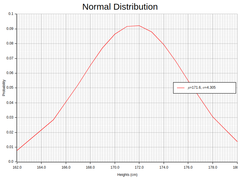
When observing, a normal distribution like the previous image illustrates, certain key properties become evident. Around 68% of data falls within one standard deviation from the mean — indicating high concentration; approximately 95% lie within two deviations — showing a wider inclusion range. Normal Distribution models random variables whose values cluster around their average value or mean accurately when graphed using the Probability Density Function (PDF) equation:

Here, x represents the value to be standardized (each height), μ represents the mean, and σ represents the standard deviation.

When measuring data, our focus is not solely on determining the quantity of a specific variable. Instead, we seek to comprehend how much it deviates from its expected or average value. This differentiation plays an essential role in evaluating variations within the data presented. To ensure that variables are comparable across different datasets, standardization (also known as normalization) is utilized to achieve this goal.

Standardization brings all factors onto comparable scales, ensuring that a single variable’s original measurement doesn’t have a disproportionate impact on the analysis or model used. This process includes subtracting the data mean and dividing it by its standard deviation. This technique establishes a standardized representation where variables are measured about their deviation from average rather than absolute values, enabling us to make more accurate comparisons across different datasets quickly!

In this way, the z-score provides valuable insight into a data point’s relative position and deviation within the distribution. The standard normal distribution, also known as the Z Distribution, is a particular type of normal distribution characterized by a mean of 0 and a standard deviation of 1. The standard normal distribution is a reference distribution, enabling us to interpret z-scores and compare different datasets easily.

To better understand the Normal Distribution, imagine having access to a large amount of data regarding the heights of individuals in a particular population. With this information, you can make well-informed decisions and draw accurate conclusions about the overall population. By analyzing this data using the normal distribution, you can calculate both mean and standard deviation values which represent average height as well as variability within that group respectively.

Now let us examine some actual numbers from our sample set: 168 cm, 172 cm,165cm ,170cm ,174cm ,180 cm, 162 cm, etc. By calculating their respective means & deviations we gain valuable insights into this specific population; allowing for compelling discussions based on concrete results!

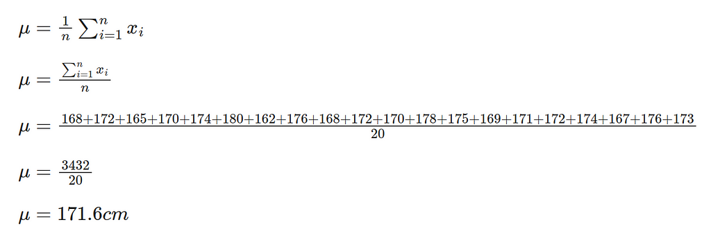
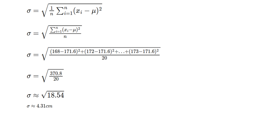
To determine the standard deviation, it is necessary to calculate the variance between every height and its mean by squaring them, adding up all these values together, dividing this sum by n-1, and finally taking the square root. Herein xi represents each individual value for height while n represents the total number of observations made.

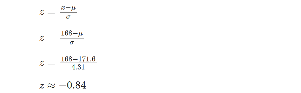
After obtaining the mean (μ) and standard deviation (σ) through prior calculations, we can proceed to determine the z-score for every height measurement by utilizing this formula:

Here, x represents the value to be standardized (each height), μ represents the mean, and σ represents the standard deviation. For example, let’s calculate the z-score for the first height value, 168:

Repeat this calculation for each height value to obtain the corresponding z-scores.

In Rust, we can perform the previous calculations using the statrs library and then plot the results using plotters. First, we need to create a heights samples vector sorted in ascending order and their corresponding probabilities. Then, we zip these two vectors into a vector of tuples, where each tuple represents a pair of height sample value and its corresponding probability.

let random_points:Vec<(f64,f64)> = {
    let heights_dist = Normal::new(171.6, 4.305).unwrap();
    let mut heights = vec![162.0, 165.0, 167.0, 168.0, 168.0, 169.0, 170.0, 170.0, 171.0, 172.0, 172.0, 172.0, 173.0, 174.0, 174.0, 175.0, 176.0, 176.0, 178.0, 180.0];
    let y_iter: Vec<f64> = heights.iter().map(|x| heights_dist.pdf(*x)).collect();
    heights.into_iter().zip(y_iter).collect()
};
println!("{:?}", random_points);

// Output:

// [(162.0, 0.0077111498014200905), (165.0, 0.0286124002877568), (167.0, 0.05236124932813138), (168.0, 0.0653262210511061), (168.0, 0.0653262210511061), (169.0, 0.07722030750534586), (170.0, 0.08648523542740724), (170.0, 0.08648523542740724), (171.0, 0.09177383324586816), (172.0, 0.09227036241240198), (172.0, 0.09227036241240198), (172.0, 0.09227036241240198), (173.0, 0.08789659179986477), (174.0, 0.07933198103903279), (174.0, 0.07933198103903279), (175.0, 0.06784080894510099), (176.0, 0.05496676666227962), (176.0, 0.05496676666227962), (178.0, 0.03069148492847293), (180.0, 0.01381024648433747)]

The 171.6 and 4.305 values in the Normal::new method represent the mean and the standard deviation values respectively, that are computed previously. Notice the heights_dist.pdf function invocation which computes the Normal distribution pdf for a given height sample.

Now, it is time to draw this vector using plotters:

evcxr_figure((640, 480), |root| {
    let mut chart = ChartBuilder::on(&root)
        .caption("Normal Distribution", ("Arial", 30).into_font())
        .x_label_area_size(40)
        .y_label_area_size(40)
        .build_cartesian_2d(162f64..180f64, 0f64..0.1f64)?;
    
    chart.configure_mesh()
        .x_desc("Heights (cm)")
        .y_desc("Probability")
        .draw()?;

    chart.draw_series(LineSeries::new(
        random_points.iter().map(|(x, y)| (*x, *y)),
        &RED
    )).unwrap()
    .label("𝜇=171.6, 𝜎=4.305")
    .legend(|(x,y)| PathElement::new(vec![(x,y), (x + 20,y)], &RED));

    chart.configure_series_labels()
        .background_style(&WHITE)
        .border_style(&BLACK)
        .draw()?;

    Ok(())
}).style("width:100%")

The above code snippet is pretty straightforward. Executing this piece of code will result in the previous image being drawn in your notebook. What is important here is this line of code:

chart.draw_series(LineSeries::new(
        random_points.iter().map(|(x, y)| (*x, *y)),
        &RED
    )).unwrap()

This creates a line from left to right using vector coordinates (height samples, x) and their corresponding probabilities (y). Explaining the code is beyond this article’s scope, but a detailed article on Plotters is coming soon. Stay tuned!

2. Binomial Distribution

Binomial outcomes are fundamental to analytics as they frequently signify the conclusion of a decision-making process. These results can encompass diverse situations, including purchase/don’t purchase, click/no-click, survival/death, and more. The crux of the binomial distribution lies in comprehending a sequence of trials where each trial has two potential outcomes with corresponding probabilities.

A binomial distribution possesses the following characteristics:

1. Number of Trials: The distribution involves a fixed number, denoted as “n”, of identical trials.
2. Two Possible Outcomes: Each trial results in only one of two possible outcomes. These outcomes can be referred to as “success” and “failure”, but they can represent any two mutually exclusive events.
3. Independence of Trials: The outcomes of one trial are independent and do not influence the outcomes of other trials. The occurrence or non-occurrence of success in one trial does not impact the probability of success in subsequent trials.
4. Constant Probability: The probability of success, represented as “p”, remains the same for each trial. Similarly, the probability of failure, denoted as “q”, is complementary to p and remains constant across trials.
5. Random Variable: The random variable in a binomial distribution represents the count or number of successes observed in the n trials. It ranges from 0 to n, inclusive, as the maximum number of successes cannot exceed the total number of trials.
6. Mean and Variance: The mean can be found by multiplying the number of trials, n, and probability of success, p. Calculating variance in this scenario is done through multiplication involving n,p, and also q which represents the probability of failure.

The formulas for mean and variance are as follows:

Mean = n * p
Variance = n * p * q = n * p * (1−p)

Let us examine a binomial experiment instance where you carry out an investigation to verify the count of individuals within a 100-member group who have cast their vote for a particular candidate in an election. In this scenario, every attempt yields either “yes” (voted for the candidate) or “no” (did not vote for the candidate).

• Step 1. Define the variables: To begin with, we need to establish the variables involved in our survey. Firstly, there were 100 individuals surveyed (n). Secondly, the probability of success, i.e., voting for a particular candidate, is denoted by p and remains unknown at this point. Thirdly, q represents the likelihood of failure or not voting for that same individual; it’s calculated as 1-p since both probabilities must add up to one. Finally, k refers to how many people voted positively towards the given candidate during our research project, which happens to be what interests us most here!
• Step 2. Estimate the probability: The likelihood of success (p) may remain unknown, encouraging you to rely on available information or presumptions for estimation. Suppose we analyze voting trends and deduce a 0.6 chance of casting votes favoring this candidate (p), implying an inverse probability value for not supporting them (q) at 0.4 instead.
• Step 3. Calculate the binomial coefficient: The binomial coefficient represents the number of ways to choose k successes out of n trials and is denoted by (k n). We can calculate it using the following formula:

• Step 4. Calculate the probability: With the binomial probability formula, we can now determine the likelihood of having precisely k individuals vote for the candidate within a group of 100.

This can be represented as:

By adjusting various k values, we can accurately calculate the probabilities linked with achieving varying numbers of respondents who have voted for the candidate in this survey. This approach empowers us to make informed decisions based on reliable data and insights.

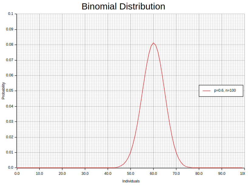
With Rust, computing the probability mass function (PMF) for our example is effortless with the aid of the statrs library. To present a clear visualization of these results in an orderly plot, we can utilize plotters library. This process involves two steps.

First and foremost, we need to create a vector called “individuals” that includes the sample values along with their corresponding probabilities. By merging these two vectors into tuples within a new vector, we can establish pairs between each trial’s value and its relevant probability. The following code serves as an excellent example of how this task can be achieved while maintaining clear variables and meaningful method calls:

let random_points:Vec<(f64,f64)> = {
    let individuals_dist = Binomial::new(0.6, 100).unwrap();
    let mut individuals: Vec<f64> = (0 .. 100).map(f64::from).collect();
    let y_iter: Vec<f64> = individuals.iter().map(|x| individuals_dist.pmf(*x as u64)).collect();
    individuals.into_iter().zip(y_iter).collect()
};

In the above code, we set the parameters for our binomial distribution (0.6 for the success probability, p, and 100 for the number of trials, n). These values are calculated beforehand and then used within the Binomial::new method. Notice the invocation of individuals_dist.pmf, which calculates the PMF for each individual based on the binomial distribution. To ensure compatibility with the Binomial::pmf method, the as u64 casting is employed, converting the floating-point numbers into unsigned 64-bit integers.

Once we have the vector random_points, we can proceed to plot it using the plotters library, as demonstrated in the accompanying notebook.

3. Geometric Distribution

The Geometric distribution is a powerful statistical technique that helps us predict the number of attempts needed to achieve success in a series of independent trials with only two possible outcomes, either success or failure. To apply this method, we must assume that each trial’s outcome does not affect subsequent ones and holds an equal probability for both success and failure. Furthermore, it presupposes that the probability mass function (PMF) adheres to this specific formula:

In this equation, x represents any one of the repeated values of the random variable X, which represents the number of trials needed until the first occurrence of a successful event A. The term (1 — p) represents the probability of an event other than A (i.e., failure), denoted as P(Ā), while p represents the probability of event A (i.e., success), denoted as P(A). Additionally, the expected value (mean) of the Geometric distribution is given by:

And the variance of the Geometric distribution is given by:

Let’s consider an example to understand the Geometric distribution application better. Suppose we flip a fair coin until we get heads for the first time. What is the probability that it takes exactly 4 flips to achieve the first head? In this case, we have a success probability of p = 0.5 since the coin is fair. We can use the Geometric distribution formula to calculate the probability:

It can be inferred that the likelihood of obtaining a head in exactly 4 flips is approximately 6.25%, as per the Geometric distribution’s application in determining probabilities linked with reaching a particular result after numerous attempts. This instance showcases how this method helps in calculating trial counts for achieving desired outcomes accurately and efficiently.

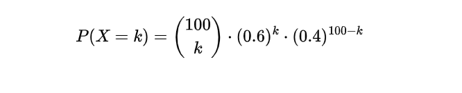
The utilization of Rust in combination with the statrs library provides a rich method for computing probability mass function (PMF) values across varying success probabilities, p. For visually appealing and impactful representations of these findings, we can rely on the plotters library. The process involves two different steps.

To begin, we create a sorted vector called “individuals” that contains the sample values for our experiment’s individuals, alongside their corresponding probabilities. By combining these two vectors into a new vector of tuples, each tuple represents a trial sample value paired with its corresponding probability. Here’s an example showcasing this process for three different probability values, 0.2, 0.5, and 0.8, using the Geometric distribution:

let random_points1:Vec<(f64,f64)> = {
    let individuals_dist = Geometric::new(0.2).unwrap();
    let mut individuals: Vec<f64> = (1 .. 10).map(f64::from).collect();
    let y_iter: Vec<f64> = individuals.iter().map(|x| individuals_dist.pmf(*x as u64)).collect();
    individuals.into_iter().zip(y_iter).collect()
};
let random_points2:Vec<(f64,f64)> = {
    let individuals_dist = Geometric::new(0.5).unwrap();
    let mut individuals: Vec<f64> = (1 .. 10).map(f64::from).collect();
    let y_iter: Vec<f64> = individuals.iter().map(|x| individuals_dist.pmf(*x as u64)).collect();
    individuals.into_iter().zip(y_iter).collect()
};
let random_points3:Vec<(f64,f64)> = {
    let individuals_dist = Geometric::new(0.8).unwrap();
    let mut individuals: Vec<f64> = (1 .. 10).map(f64::from).collect();
    let y_iter: Vec<f64> = individuals.iter().map(|x| individuals_dist.pmf(*x as u64)).collect();
    individuals.into_iter().zip(y_iter).collect()
};

In the above code, we initialize three sets of random_points, each corresponding to a different probability of success, p, in the Geometric distribution. Note how we invoke the individuals_dist.pmf function, which calculates the PMF for a given trial based on the Geometric distribution. To ensure compatibility with the Geometric::pmf method, we use the as u64 casting, converting the floating-point numbers into unsigned 64-bit integers.

Now we can plot this vector using plotters as shown in the accompanying notebook.

4. Hypergeometric Distribution

The Hypergeometric Distribution is a probability distribution that shares similarities with the binomial distribution. It’s used to model the likelihood of success in a hypergeometric experiment, where specific properties must be met. Firstly, random selection occurs when taking a sample size of n from population N without replacement. Secondly, M represents the number of successes within this population, and thirdly (N — M) denotes failures. Using these three characteristics as guidelines for experimentation, we can define an equation that gives us our Probability Density Function (PDF).

In this equation, X represents the random variable, and x represents the number of observed (sample) successes. Let’s consider the following example: Suppose there is a bag containing 100 marbles, out of which 20 marbles are red and 80 marbles are blue. We randomly select 10 marbles from the bag without replacement. We want to calculate the probability of obtaining exactly 3 red marbles.

To calculate the probability, we can utilize the Hypergeometric Distribution. Let’s define the variables:

• N = Total number of marbles in the bag = 100
• K or M = Number of red marbles in the bag = 20
• n = Number of marbles drawn = 10
• k = Number of red marbles drawn = 3

Now, let’s calculate the probability of drawing exactly k=3 red marbles:

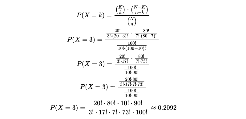
The result indicates that the probability of drawing exactly 3 red marbles out of the 10 marbles selected is approximately 0.2092, or 20.92%. This probability quantifies the likelihood of obtaining this specific outcome.

Through the utilization of Hypergeometric distribution, we can compute the probabilities linked to different situations that occur when sampling without replacement from a finite population. This technique enables us to analyze and comprehend with clarity various combinations’ likelihoods, thereby making informed decisions based on calculated probabilities.

It is important to remember that the Hypergeometric distribution plays a crucial role in analyzing the probability of specific outcomes within a finite population, without any replacement. This statistical technique holds immense significance across diverse fields like genetics, quality control and market research where sampling methods are restricted by limited resources or individuals.

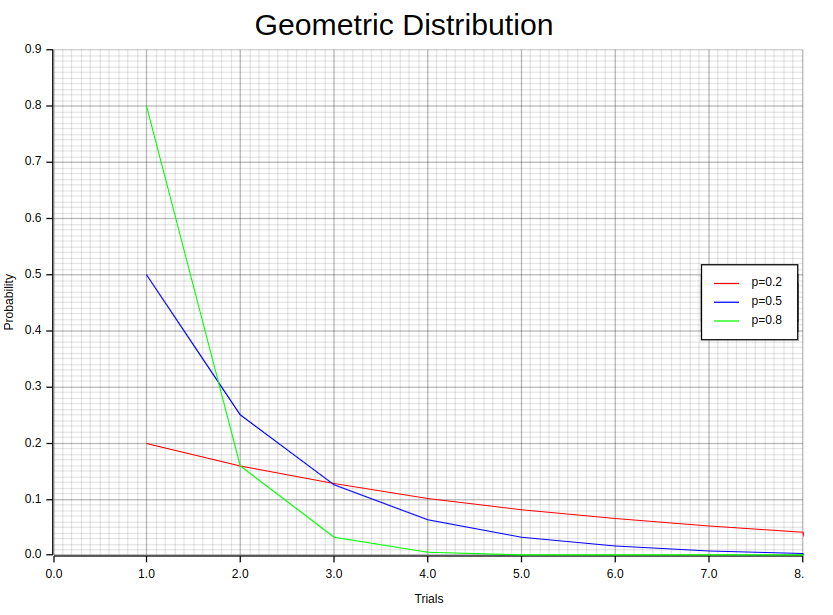
In Rust, we can compute the probability mass function (PMF) for different values for the (N, M, n) triplet using statrs library and then plot the results using plotters. First, we need to create an “individuals” samples vector sorted in ascending order and their corresponding probabilities. Then, we zip these two vectors into a vector of tuples, where each tuple represents a pair of trial sample value and its corresponding probability.

let random_points1:Vec<(f64,f64)> = {
    let individuals_dist = Hypergeometric::new(500, 50, 100).unwrap();
    let mut individuals: Vec<f64> = (0 .. 60).map(f64::from).collect();
    let y_iter: Vec<f64> = individuals.iter().map(|x| individuals_dist.pmf(*x as u64)).collect();
    individuals.into_iter().zip(y_iter).collect()
};
let random_points2:Vec<(f64,f64)> = {
    let individuals_dist = Hypergeometric::new(500, 60, 200).unwrap();
    let mut individuals: Vec<f64> = (0 .. 60).map(f64::from).collect();
    let y_iter: Vec<f64> = individuals.iter().map(|x| individuals_dist.pmf(*x as u64)).collect();
    individuals.into_iter().zip(y_iter).collect()
};
let random_points3:Vec<(f64,f64)> = {
    let individuals_dist = Hypergeometric::new(500, 70, 300).unwrap();
    let mut individuals: Vec<f64> = (0 .. 60).map(f64::from).collect();
    let y_iter: Vec<f64> = individuals.iter().map(|x| individuals_dist.pmf(*x as u64)).collect();
    individuals.into_iter().zip(y_iter).collect()
};

The 500, 50, 100 values in eachHypergeometric::new method represents the population (N), successes (K or M), draws (n) respectively. Notice the individuals_dist.pmf function invocation which computes the Hypergeometric distribution pmf for a given trial. The as u64 in the parameter is used to cast floating point numbers to unsigned integers because the Hypergeometric::pmf method accepts 64-bit unsigned integer as parameter.

Now we can plot this vector using plotters as shown in the accompanying notebook.

5. Poisson Distribution

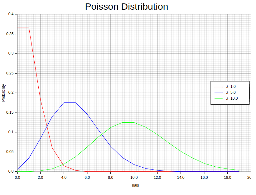
The Poisson distribution is a method of modeling the frequency of events that take place within a given timeframe, distance, area, or volume. It empowers us to understand and anticipate event occurrences by utilizing their average rate. The Probability Mass Function (PMF) plays a crucial role in determining the likelihood of specific events occurring under this model, its formula being:

In this equation, P(x=r) represents the probability of the event occurring r times, λ represents the average or expected number of occurrences, and e is the base of the natural logarithm.

The Poisson distribution can be utilized in multiple situations. For example, It allows us to determine the frequency of restaurant customers arriving per hour, count work-related accidents happening at a factory over an entire year or even assess customer complaints received by call centers on a weekly basis.

Here are some key properties of the Poisson distribution:

1. The Poisson distribution exhibits a unique relationship between its mean and variance, represented by the same value known as λ.
2. Events modeled under the Poisson distribution possess vital characteristics such as independence, randomness, and exclusivity from co-occurring.
3. Under certain conditions where n is large (typically n >20) and p is small (typically p < 0.1), substituting λ = np allows for an approximation to be made towards binomial distributions using the Poisson distribution instead.
4. In cases where n is significant in size while p is around 0.5, with a product np being more significant than 0.5, normal distributions can serve as suitable approximations when modeling data.

While skewed at first glance, it’s worth noting that increasing values of lambda result in shapes resembling those found within standard curves; the above image provides visual evidence supporting this claim!

Let’s work through a solved example to illustrate the application of the Poisson distribution. The average number of defective products per hour in a manufacturing facility is five. Assuming that the number of defects follows a Poisson distribution, let’s calculate the probability of the following scenarios:

• Exactly eight defective products in one hour:

P(x=8) = (e^(-5) * 5⁸) / 8! = 0.06527803934815865

• No more than three defective products in one hour:

P(x<=3) = P(x=0) + P(x=1) + P(x=2) + P(x=3) = 0.7349740847026385

By substituting the appropriate values into the Poisson PMF equation and performing the calculations, we can determine the probabilities associated with these specific situations in the manufacturing facility. This information can be valuable for quality control and decision-making purposes, allowing us to assess the likelihood of encountering different numbers of defective products within a given timeframe.

In Rust, we can compute the probability mass function (PMF) for different values of λ using statrs library and then plot the results using plotters. First, we need to create an “individuals” samples vector sorted in ascending order and their corresponding probabilities. Then, we zip these two vectors into a vector of tuples, where each tuple represents a pair of trial sample value and its corresponding probability.

let random_points1:Vec<(f64,f64)> = {
    let individuals_dist = Poisson::new(1.0).unwrap();
    let mut individuals: Vec<f64> = (0 .. 20).map(f64::from).collect();
    let y_iter: Vec<f64> = individuals.iter().map(|x| individuals_dist.pmf(*x as u64)).collect();
    individuals.into_iter().zip(y_iter).collect()
};
let random_points2:Vec<(f64,f64)> = {
    let individuals_dist = Poisson::new(5.0).unwrap();
    let mut individuals: Vec<f64> = (0 .. 20).map(f64::from).collect();
    let y_iter: Vec<f64> = individuals.iter().map(|x| individuals_dist.pmf(*x as u64)).collect();
    individuals.into_iter().zip(y_iter).collect()
};
let random_points3:Vec<(f64,f64)> = {
    let individuals_dist = Poisson::new(10.0).unwrap();
    let mut individuals: Vec<f64> = (0 .. 20).map(f64::from).collect();
    let y_iter: Vec<f64> = individuals.iter().map(|x| individuals_dist.pmf(*x as u64)).collect();
    individuals.into_iter().zip(y_iter).collect()
};

The 1.0, 5.0, 10.0 values in each Poisson::new method represents different values of λ. Notice the individuals_dist.pmf function invocation which computes the Poisson distribution pmf for a given trial. The as u64 in the parameter is used to cast floating point numbers to unsigned integers because the Poisson::pmf method accepts 64-bit unsigned integer as parameter.

Now we can plot this vector using plotters as shown in the accompanying notebook.

6. Exponential Distribution

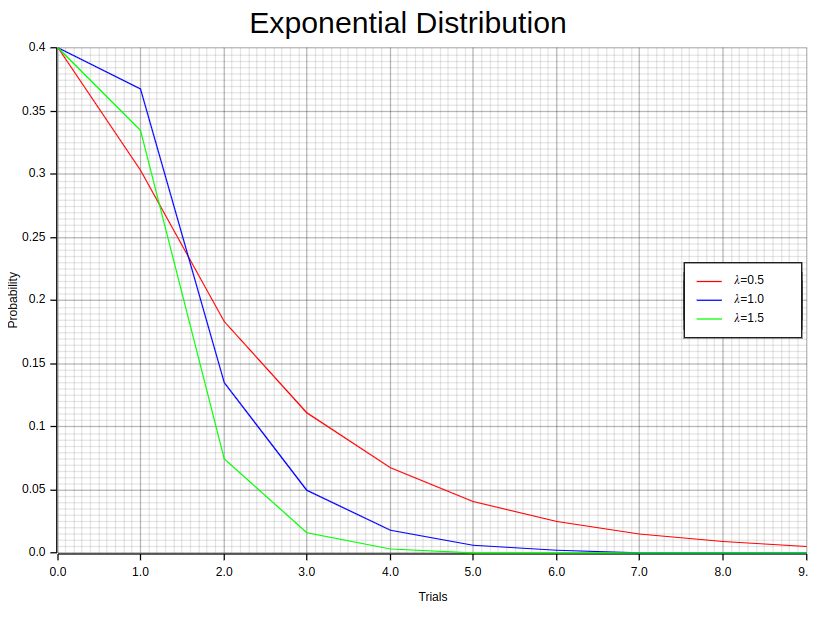
The negative exponential distribution, also referred to as the exponential distribution, is a widely utilized probability model for calculating time intervals between events in Poisson processes. Its versatility has made it an essential tool across several fields including survival analysis, queuing theory, and reliability analysis. The probability density function of this distribution is given by the following equation:

The parameter λ and variable x signify the rate and the duration between events, respectively. The exponential distribution provides a remarkable attribute — a consistent hazard rate, indicating that an event’s probability remains constant regardless of how much time has passed. To express this distribution mathematically, we use the cumulative distribution function represented by this equation:

The probability density and cumulative distribution function graphs illustrate the exponential distribution. The PDF graph displays a decaying exponential curve, which implies that shorter intervals between events have higher chances of occurring. On the other hand, the CDF graph starts from 0 and gradually approaches 1 as time progresses to signify how probabilities accumulate over time.

To illustrate this distribution, suppose we are studying the arrival times of customers at a coffee shop. Based on historical data, it is known that customers arrive at an average rate of 10 customers per hour, following an Exponential distribution. We want to analyze the probability of specific waiting times between customer arrivals.

Let us consider the scenario where we need to determine the likelihood of waiting precisely 30 mins (0.5 hr) between two consecutive customer arrivals. To achieve this, we can utilize the Probability Density Function associated with this distribution which is expressed as:

where λ is the rate parameter and x is the waiting time. Substituting the given values into the equation, we have:

Simplifying further, we get:

Performing the calculation:

The calculated probability, ~ 0.0673, indicates the likelihood of experiencing a 0.5 hour between customer arrivals, based on the Exponential distribution with an average arrival rate of 10 customers per hour.

In essence, the Exponential distribution can be utilized to analyze waiting times and gain insights into the likelihoods related to particular time frames. This example highlights its practical application, demonstrating how it facilitates a deeper understanding of such probabilities.

In Rust, we can compute the probability density function (PDF) for different values of λ using statrs library and then plot the results using plotters. First, we need to create an “individuals” samples vector sorted in ascending order and their corresponding probabilities. Then, we zip these two vectors into a vector of tuples, where each tuple represents a pair of trial sample value and its corresponding probability.

let random_points1:Vec<(f64,f64)> = {
    let individuals_dist = Exp::new(0.5).unwrap();
    let mut individuals: Vec<f64> = (0 .. 10).map(f64::from).collect();
    let y_iter: Vec<f64> = individuals.iter().map(|x| individuals_dist.pdf(*x)).collect();
    individuals.into_iter().zip(y_iter).collect()
};
let random_points2:Vec<(f64,f64)> = {
    let individuals_dist = Exp::new(1.0).unwrap();
    let mut individuals: Vec<f64> = (0 .. 10).map(f64::from).collect();
    let y_iter: Vec<f64> = individuals.iter().map(|x| individuals_dist.pdf(*x)).collect();
    individuals.into_iter().zip(y_iter).collect()
};
let random_points3:Vec<(f64,f64)> = {
    let individuals_dist = Exp::new(1.5).unwrap();
    let mut individuals: Vec<f64> = (0 .. 10).map(f64::from).collect();
    let y_iter: Vec<f64> = individuals.iter().map(|x| individuals_dist.pdf(*x)).collect();
    individuals.into_iter().zip(y_iter).collect()
};

The 0.5, 1.0, 1.5 values in each Exp::new method represents different values of λ. Notice the individuals_dist.pdf function invocation which computes the Exponential distribution pdf for a given sample.

Now we can plot this vector using plotters as shown in the accompanying notebook.

7. Gamma Distribution

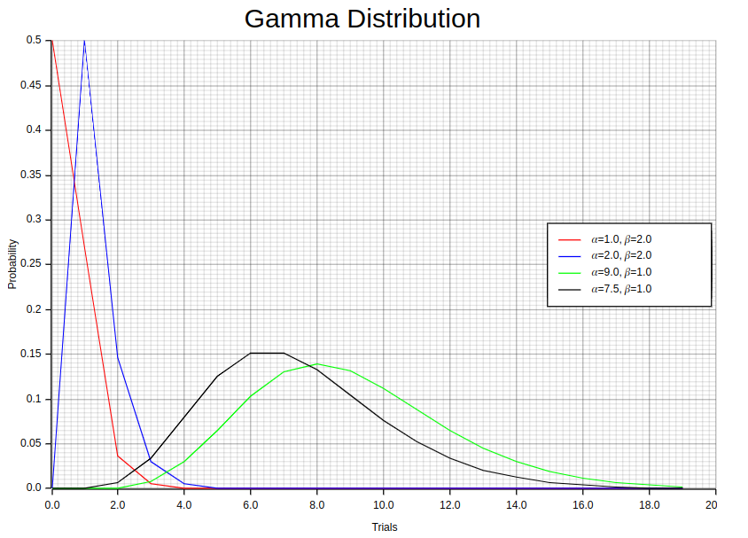
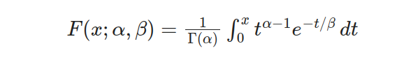
The Gamma distribution is a continuous probability distribution with numerous applications in diverse fields like finance, climatology services, and queuing models. It offers an adequate mathematical model for determining the likelihood of observing various values within an indefinite range. This type of distribution proves particularly useful when handling skewed data with non-negative values. Its defining features include its cumulative distribution function (CDF) and probability density function (PDF), which can be defined using different parameters to suit specific needs.

The Gamma distribution, which has a single parameter, stands out as an individual variation within the vast Gamma family. Its probability density function (PDF) sets it apart and can be represented by this formula:

In this equation, α represents the shape parameter of the distribution, which determines the skewness and shape of the curve. The term Γ(α) refers to the gamma function.

The gamma function serves as a vital normalizing factor in the probability density function (PDF), guaranteeing that the total area beneath its curve equals 1. This crucial component plays a significant role in determining probabilities and quantiles linked to the Gamma distribution’s one-parameter calculations.

The General Gamma distribution also referred to as the two-parameter Gamma distribution, extends the one-parameter Gamma (γ) by incorporating an additional scale parameter (β). By including this parameter, the PDF of the two-parameter Gamma distribution can be defined as:

In this equation, α represents the shape parameter, determining the shape and skewness of the distribution, while β represents the scale parameter, influencing the spread and location of the distribution. The inclusion of β allows for greater flexibility in modeling various data sets.

It is crucial to take into account the cumulative distribution function (CDF) of the two-parameter Gamma distribution. This function indicates the likelihood that a random variable from this particular distribution will be less than or equal to any given value. Expressing it as follows:

The variable x is often employed to denote a random value in mathematical equations. Meanwhile, α and β are used as shape and scale parameters. To calculate integrals within the range of 0 to x, we use an incomplete gamma function represented by Γ(α,x/β).

To better understand the Gamma Distribution, Suppose we have a manufacturing process that produces electronic components, and the time it takes for a component to fail follows a gamma distribution. This distribution is commonly used to model the lifespan or time to failure of various types of products.

In this example, we will examine the gamma distribution with a shape parameter (α) of 2.5, implying moderate skewness, and a scale parameter (β) of 100 representing average failure time. By utilizing the gamma distribution, it is possible to determine probabilities linked to specific events in this scenario. For instance, we can calculate the likelihood of an element failing within its first 50 hours:

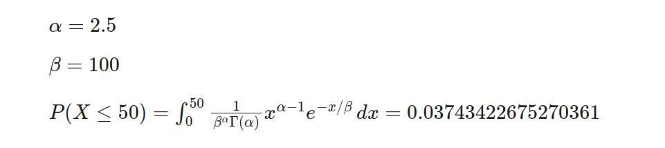
The probability of a component lasting more than 200 hours:

These calculations offer valuable knowledge regarding the durability and lifespan of manufactured electronic parts. Manufacturers can make well-informed decisions concerning product warranties, maintenance routines, and quality control measures by comprehending the likelihoods linked to failure times.

In Rust, we can compute the probability density function (PDF) for different values of the shape parameter (α) and scale parameter (β) using statrs library and then plot the results using plotters. First, we need to create an “individuals” samples vector sorted in ascending order and their corresponding probabilities. Then, we zip these two vectors into a vector of tuples, where each tuple represents a pair of trial sample value and its corresponding probability.

let random_points1:Vec<(f64,f64)> = {
    let individuals_dist = Gamma::new(1.0, 2.0).unwrap();
    let mut individuals: Vec<f64> = (0 .. 20).map(f64::from).collect();
    let y_iter: Vec<f64> = individuals.iter().map(|x| individuals_dist.pdf(*x)).collect();
    individuals.into_iter().zip(y_iter).collect()
};
let random_points2:Vec<(f64,f64)> = {
    let individuals_dist = Gamma::new(2.0, 2.0).unwrap();
    let mut individuals: Vec<f64> = (0 .. 20).map(f64::from).collect();
    let y_iter: Vec<f64> = individuals.iter().map(|x| individuals_dist.pdf(*x)).collect();
    individuals.into_iter().zip(y_iter).collect()
};
let random_points3:Vec<(f64,f64)> = {
    let individuals_dist = Gamma::new(9.0, 1.0).unwrap();
    let mut individuals: Vec<f64> = (0 .. 20).map(f64::from).collect();
    let y_iter: Vec<f64> = individuals.iter().map(|x| individuals_dist.pdf(*x)).collect();
    individuals.into_iter().zip(y_iter).collect()
};
let random_points4:Vec<(f64,f64)> = {
    let individuals_dist = Gamma::new(7.5, 1.0).unwrap();
    let mut individuals: Vec<f64> = (0 .. 20).map(f64::from).collect();
    let y_iter: Vec<f64> = individuals.iter().map(|x| individuals_dist.pdf(*x)).collect();
    individuals.into_iter().zip(y_iter).collect()
};

The 1.0, 2.0 values in each Gamma::new method represents different values of the shape parameter (α) and scale parameter (β) respectively. Notice the individuals_dist.pdf function invocation which computes the Gamma distribution pdf for a given sample.

Now we can plot this vector using plotters as shown in the accompanying notebook.

8. Chi-Squared Distribution

The Chi-squared distribution is a highly effective probability distribution that finds extensive use in various statistical applications. Its greatest strength lies in its remarkable precision when it comes to analyzing data and conducting hypothesis tests. The Probability Density Function formula of this distribution can be described as follows:

The Chi-squared Distribution’s shape and characteristics are determined by an equation that involves x as the random variable, while k is an integer parameter responsible for setting degrees of freedom. To determine probabilities linked to this distribution, we use its cumulative distribution function (CDF). This CDF can be expressed through the following equation:

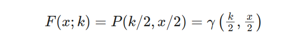
By utilizing equations that encompass diverse mathematical functions like γ(s,t), P(s,t) and Γ(k/2), it is feasible to determine the probability of a Chi-squared random variable being less than or equal to x, with k degrees of freedom. This method encompasses evaluating these equations meticulously for exact estimation of likelihood.

The Chi-squared Distribution is widely employed in various statistical analyses due to its versatile applications. Some common uses include:

1. Calculating the confidence intervals for population standard deviation of a normal distribution by utilizing sample standard deviation.
2. Evaluating the independence between two criteria while classifying multiple qualitative variables.
3. Analyzing associations and dependencies among categorical variables to reveal relationships.
4. Investigating sample variance under an assumed normal underlying distribution.
5. Examining differences in observed versus expected frequencies within categorical data through hypothesis testing.
6. Conducting a chi-square test, also known as the goodness-of-fit test, to evaluate conformity between theoretical distributions and actual observations.

The Chi-squared Distribution plays a fundamental role in these statistical analyses, providing insights into the variability and relationships within datasets.

Let’s consider an example to gain a deeper comprehension of the Chi-squared distribution. Imagine we are surveying to analyze people’s preferred mode of transportation within a city. We aim to determine whether there exists any correlation between age groups and their favored means of getting around town. We categorize our participants into three different age brackets: “Young” (18 to 30 years), “Middle-aged” (31–50 years), and “Senior” (51+). Let’s consider a hypothetical dataset with the following contingency table:

We must determine crucial elements like the Chi-Squared metric, p-value, degrees of freedom, and anticipated frequencies to carry out a Chi-Squared test. These vital components require specific calculations to ensure precise outcomes. Here are a few significant equations that aid in achieving accurate results:

• Equation 1: Calculate the Chi-Squared Statistic.

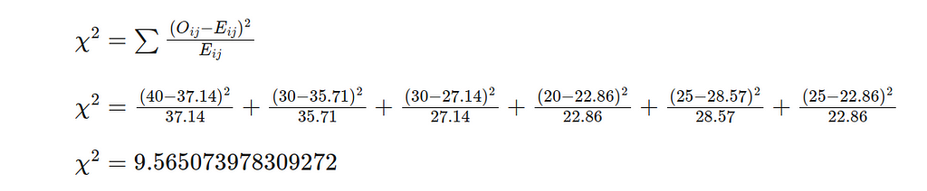
• Equation 2: Calculate the Degrees of Freedom.

• Equation 3: Calculate the p-value.

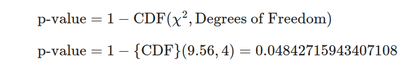
With the help of these formulas, we can manually determine the values by replacing observed frequencies from the contingency table. However, it’s important to note that this process may be complex and time-consuming; hence, statistical libraries, like Statrs, are highly recommended for precise and efficient computation.

The utilization of the Chi-Squared distribution and its associated test is exemplified in the previous example, showcasing how it can be employed to analyze categorical data and investigate correlations between variables. Through comprehending these connections, we can acquire valuable insight into the preferences and actions of diverse demographic clusters.

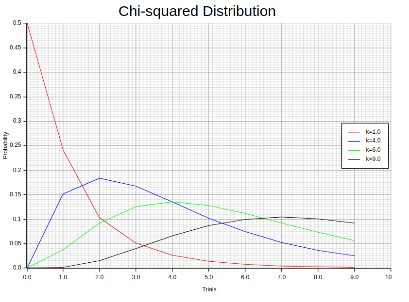
In Rust, we can compute the probability density function (PDF) for different values of the Degrees of Freedom using statrs library and then plot the results using plotters. First, we need to create an “individuals” samples vector sorted in ascending order and their corresponding probabilities. Then, we zip these two vectors into a vector of tuples, where each tuple represents a pair of trial sample value and its corresponding probability.

let random_points1:Vec<(f64,f64)> = {
    let individuals_dist = ChiSquared::new(1.0).unwrap();
    let mut individuals: Vec<f64> = (0 .. 10).map(f64::from).collect();
    let y_iter: Vec<f64> = individuals.iter().map(|x| individuals_dist.pdf(*x)).collect();
    individuals.into_iter().zip(y_iter).collect()
};
let random_points2:Vec<(f64,f64)> = {
    let individuals_dist = ChiSquared::new(4.0).unwrap();
    let mut individuals: Vec<f64> = (0 .. 10).map(f64::from).collect();
    let y_iter: Vec<f64> = individuals.iter().map(|x| individuals_dist.pdf(*x)).collect();
    individuals.into_iter().zip(y_iter).collect()
};
let random_points3:Vec<(f64,f64)> = {
    let individuals_dist = ChiSquared::new(6.0).unwrap();
    let mut individuals: Vec<f64> = (0 .. 10).map(f64::from).collect();
    let y_iter: Vec<f64> = individuals.iter().map(|x| individuals_dist.pdf(*x)).collect();
    individuals.into_iter().zip(y_iter).collect()
};
let random_points4:Vec<(f64,f64)> = {
    let individuals_dist = ChiSquared::new(9.0).unwrap();
    let mut individuals: Vec<f64> = (0 .. 10).map(f64::from).collect();
    let y_iter: Vec<f64> = individuals.iter().map(|x| individuals_dist.pdf(*x)).collect();
    individuals.into_iter().zip(y_iter).collect()
};

The 1.0, 4.0, 6.0, 9.0 values in each ChiSquared::new method represents different values of the Degrees of Freedom. Notice the individuals_dist.pdf function invocation which computes the Chi-squared distribution pdf for a given sample.

Now we can plot this vector using plotters as shown in the accompanying notebook.

9. Beta Distribution

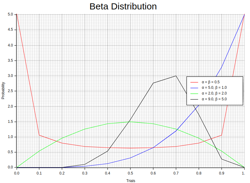
The Beta distribution is characterized by its probability density function (PDF), which is given by the following equation:

The parameters determine the distribution’s shape α and β, while a and b define the random variable x’s possible values. The beta function B(α, β) is a normalization factor in guaranteeing that the PDF integrates over the given range equals 1.

By setting the lower limit, a, to 0 and upper limit b to 1, we can simplify the Beta distribution into what is known as Standard Beta Distribution. This transformation leads us to an equation that defines its probability density function(PDF).

The Standard Beta Distribution proves to be highly beneficial when dealing with proportions or probabilities. It presents a versatile and understandable model within the [0, 1] range. Additionally, the cumulative distribution function (CDF) for this type of distribution refers to the probability that an arbitrary variable x will take on a value equal to or less than any given threshold. The CDF formula pertaining specifically to this probability density function can be expressed as follows:

The incomplete beta function ratio, also known as I_x(α, β), is represented by B_x(α, β) in this equation. By calculating the probability of observing values up to a certain threshold through the CDF, valuable insights into distribution can be obtained. It should be noted that while not explicitly provided in this text are the beta function B(α,β) and incomplete beta function ratio I_x (α, β). However mathematical libraries or packages may provide assistance for computing these functions.

To better understand the Beta distribution, Suppose we are analyzing the effectiveness of a new drug in treating a certain medical condition. The response rate to the drug follows a beta distribution with shape parameters α = 4 and β = 3. We are interested in determining the probability that the drug achieves a response rate between 60% and 70%. To compute the probability of the drug achieving a response rate between 60% and 70%, we can use the following equations:

• Step 1: Compute the cumulative distribution function (CDF) values at the upper and lower bounds:

• Step 2: Substitute the values for the lower and upper bounds, as well as the shape parameters:

• Step 3: Calculate the integral using the beta CDF formula:

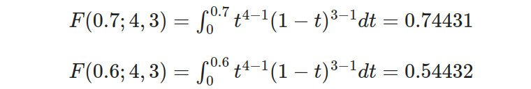
• Step 4: Calculate the probability by subtracting the lower CDF from the upper CDF:

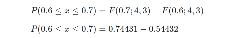
So, the probability of the drug achieving a response rate between 60% and 70% is 0.19999.

In Rust, we can compute the probability density function (PDF) for different values of the distribution’s shape α and β using statrs library and then plot the results using plotters. First, we need to create an “trials” samples vector sorted in ascending order and their corresponding probabilities. Then, we zip these two vectors into a vector of tuples, where each tuple represents a pair of trial sample value and its corresponding probability.

let random_points1:Vec<(f64,f64)> = {
    let dist = Beta::new(0.5, 0.5).unwrap();
    let mut trials: Vec<f64> = vec![0.0, 0.1, 0.2, 0.3, 0.4, 0.5, 0.6, 0.7, 0.8, 0.9, 1.0];
    let y_iter: Vec<f64> = trials.iter().map(|x| dist.pdf(*x)).collect();
    trials.into_iter().zip(y_iter).collect()
};
let random_points2:Vec<(f64,f64)> = {
    let dist = Beta::new(5.0, 1.0).unwrap();
    let mut trials: Vec<f64> = vec![0.0, 0.1, 0.2, 0.3, 0.4, 0.5, 0.6, 0.7, 0.8, 0.9, 1.0];
    let y_iter: Vec<f64> = trials.iter().map(|x| dist.pdf(*x)).collect();
    trials.into_iter().zip(y_iter).collect()
};
let random_points3:Vec<(f64,f64)> = {
    let dist = Beta::new(2.0, 2.0).unwrap();
    let mut trials: Vec<f64> = vec![0.0, 0.1, 0.2, 0.3, 0.4, 0.5, 0.6, 0.7, 0.8, 0.9, 1.0];
    let y_iter: Vec<f64> = trials.iter().map(|x| dist.pdf(*x)).collect();
    trials.into_iter().zip(y_iter).collect()
};
let random_points4:Vec<(f64,f64)> = {
    let dist = Beta::new(9.0, 5.0).unwrap();
    let mut trials: Vec<f64> = vec![0.0, 0.1, 0.2, 0.3, 0.4, 0.5, 0.6, 0.7, 0.8, 0.9, 1.0];
    let y_iter: Vec<f64> = trials.iter().map(|x| dist.pdf(*x)).collect();
    trials.into_iter().zip(y_iter).collect()
};

Each pair of values (e.g. (0.5, 0.5)) in each Beta::new method represents different values of the distribution’s shape α and β. Notice the dist.pdf function invocation which computes the Beta distribution pdf for a given sample.

Now we can plot this vector using plotters as shown in the accompanying notebook.

10. Negative Binomial Distribution

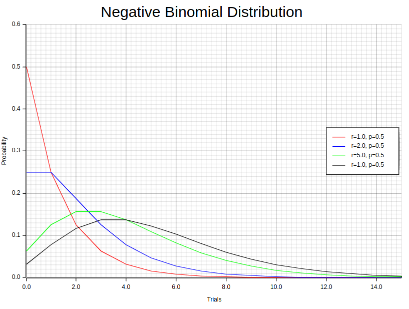
The concept of “negative” numbers is entirely unrelated to the distribution we discuss in this section. Let’s delve into the nature of this distribution by considering an experiment composed of a series of x-repeated trials. In this experiment, each trial stands independently, meaning that the outcome of one trial does not influence or depend on the outcomes of the other trials. Crucially, these trials have only two possible outcomes: success or failure. It is important to note that the probability of success remains constant and consistent across all trials. Mathematically, we can express this distribution through a well-defined equation as follows:

In this equation, x symbolizes the total number of trials conducted in the experiment. Meanwhile, r represents the number of successes observed throughout these trials. The term P(x,r,p) denotes the negative binomial probability, which measures the likelihood of obtaining a specific number of successes in a given number of trials. Lastly, p signifies the probability of success on an individual trial, while (1-p) represents the probability of failure on an individual trial.

Interestingly, there are special cases where the negative binomial distribution aligns with the geometric distribution. Specifically, we observe this equivalence when the number of successes (r) is set to 1. As we discussed previously, geometric distribution, in essence, represents the probability distribution for the number of trials required to achieve the first success in a series of independent trials. Therefore, in situations where r equals 1, the negative binomial distribution can be mathematically equivalent to the geometric distribution. The example graphs presented above clearly demonstrate this special connection between the two distributions.

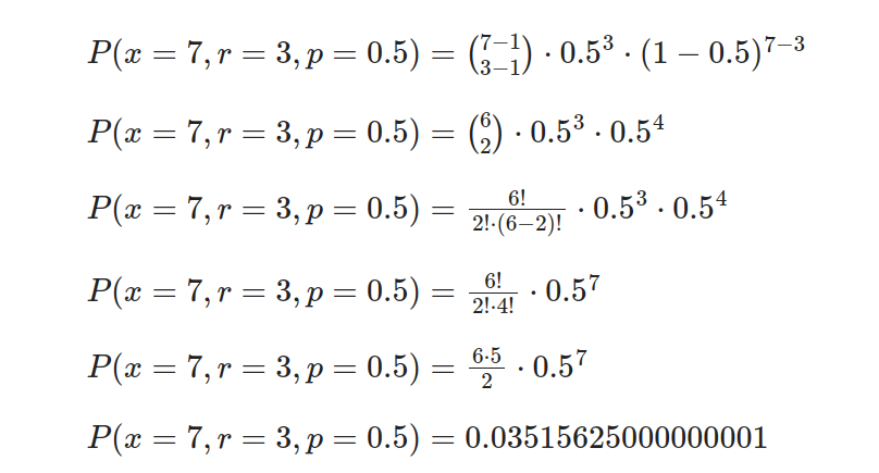
To better understand this distribution, suppose we are conducting a series of independent coin flips and want to determine the probability of obtaining the third consecutive heads on the seventh flip. Let’s calculate this probability using the negative binomial distribution.

Consider this example: the likelihood of obtaining heads on each toss (p) is 0.5, and our focus lies in achieving three successes overall (r) during seven consecutive flips (x).

• Step 1: Define the variables.

- Probability of success (p): 0.5
- Number of trials (x): 7
- Number of successes (r): 3

• Step 2: Calculate the negative binomial probability.

Substitute the values into the formula and calculate the probability.

In Rust, we can compute the Probability Mass Function (PMF) for different values of r, the number of successes and p, the probability of success using statrs library and then plot the results using plotters. First, we need to create an “trials” samples vector sorted in ascending order and their corresponding probabilities. Then, we zip these two vectors into a vector of tuples, where each tuple represents a pair of trial sample value and its corresponding probability.

let random_points1:Vec<(f64,f64)> = {
    let dist = NegativeBinomial::new(1.0, 0.5).unwrap();
    let mut trials: Vec<f64> = (0 .. 25).map(f64::from).collect();
    let y_iter: Vec<f64> = trials.iter().map(|x| dist.pmf(*x as u64)).collect();
    trials.into_iter().zip(y_iter).collect()
};
let random_points2:Vec<(f64,f64)> = {
    let dist = NegativeBinomial::new(2.0, 0.5).unwrap();
    let mut trials: Vec<f64> = (0 .. 25).map(f64::from).collect();
    let y_iter: Vec<f64> = trials.iter().map(|x| dist.pmf(*x as u64)).collect();
    trials.into_iter().zip(y_iter).collect()
};
let random_points3:Vec<(f64,f64)> = {
    let dist = NegativeBinomial::new(4.0, 0.5).unwrap();
    let mut trials: Vec<f64> = (0 .. 25).map(f64::from).collect();
    let y_iter: Vec<f64> = trials.iter().map(|x| dist.pmf(*x as u64)).collect();
    trials.into_iter().zip(y_iter).collect()
};
let random_points4:Vec<(f64,f64)> = {
    let dist = NegativeBinomial::new(5.0, 0.5).unwrap();
    let mut trials: Vec<f64> = (0 .. 25).map(f64::from).collect();
    let y_iter: Vec<f64> = trials.iter().map(|x| dist.pmf(*x as u64)).collect();
    trials.into_iter().zip(y_iter).collect()
};

Each pair of values (e.g. (1.0, 0.5)) in each NegativeBinomial::new method represents different values of r, the number of successes and p, the probability of success. Notice the dist.pmf function invocation which computes the Negative Binomial distribution pmf for a given sample.

Now we can plot this vector using plotters as shown in the accompanying notebook.

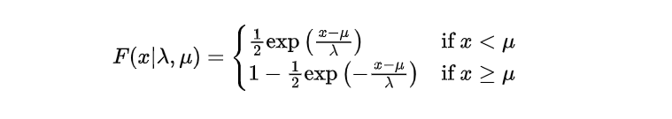
11. Laplace Distribution

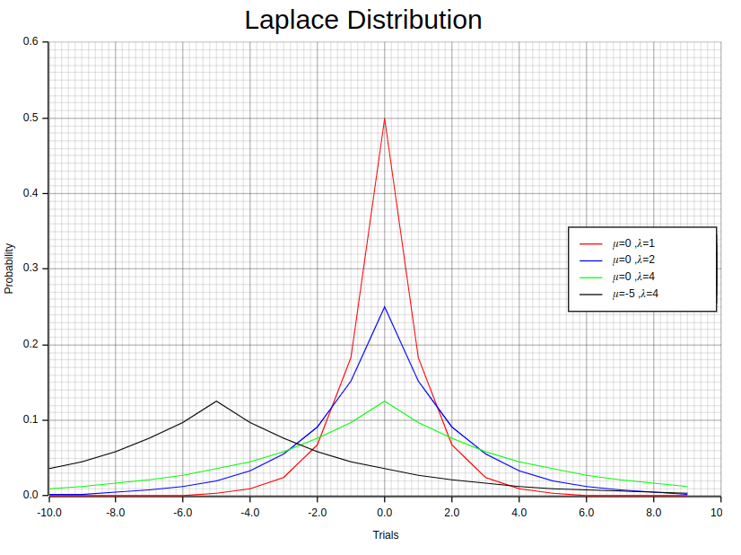
The Laplace distribution, also known as the double exponential distribution, exhibits distinct characteristics that set it apart. When we delve into the one-parameter Laplace distribution, its probability density function can be elegantly expressed through the following equation:

Within this equation, the scale parameter λ plays a pivotal role, governing the spread and width of the distribution. It quantifies the magnitude of the fluctuations and how the data is dispersed.

To better understand the one-parameter Laplace distribution, we will delve into its corresponding cumulative distribution function (CDF). The CDF offers valuable information on the accumulated probabilities linked with various random variable values. Specifically for this type of distribution, we can express its CDF mathematically as:

This CDF is constructed to handle both positive and negative values of the random variable x, with the scale parameter λ controlling the rate at which the probabilities accumulate.

Expanding our understanding to encompass the two-parameter Laplace distribution, we encounter additional parameters influencing its behavior. The probability density function (PDF) for the two-parameter Laplace distribution can be formulated as follows:

In this case, the scale parameter λ still determines the dispersion of the distribution. In contrast, the location parameter μ denotes the central point or location around which the data tend to cluster. The interplay between λ and μ enables flexible and versatile data modeling.

Just like the single-parameter Laplace distribution, its two-parameter counterpart also has a cumulative distribution function (CDF). This CDF represents the cumulative probabilities associated with different values of the random variable. Specifically for the two-parameter Laplace distribution, this CDF can be denoted as:

The structure of this CDF enables it to adapt both positive and negative values for the random variable x. The scale parameter λ plays a vital role in regulating the probability accumulation pace.

In addition to the distributional properties, this distribution possesses certain statistical moments. The location parameter straightforwardly gives the expected value (mean) of the Laplace distribution.

The equation suggests that the anticipated value aligns with the distribution’s midpoint, signifying a standard or mean measurement of the random variable. Additionally, it is possible to determine the Laplace distribution’s variance by computing:

The extent to which a distribution is scattered or dispersed around the average value can be determined by its variance. When it comes to Laplace’s probability density function, the magnitude of λ directly correlates with the square of its scale parameter. It hence influences how much spread there will be in data points. Therefore, an increase in λ would result in more significant variability and wider dispersion within this type of distribution.

Using example plots is a common practice to visually represent the probability density function (PDF) of a one-parameter Laplace distribution with parameters (λ, 0). These plots effectively convey information about the shape and features of this particular distribution. By examining its PDF form, we can get valuable insights into how probable it is for various values to occur within this specific distribution.

By analyzing these plots, we can comprehensively understand the distribution’s pattern and tendencies. The influence that λ, the scale parameter, has on both symmetry and spread is emphasized through this examination.

Suppose we have a manufacturing process that produces electronic components. The time it takes for a component to fail follows a Laplace distribution with a location parameter μ=10 and a scale parameter λ=2. We want to compute the probability that a component will fail in the [8, 12] hours interval after production. The Laplace distribution probability density function (PDF) is given by:

To find the cumulative probability, we integrate the PDF from negative infinity to a given value x:

The cumulative distribution function is defined as follows:

Given our parameters of μ=10 and λ=2, we aim to determine the probability that the component will malfunction within a time frame spanning from 8 to 12 hours. This can be mathematically represented as:

Substituting the values into the equation, we have:

Simplifying further:

Finally, we evaluate the expression to obtain the result:

We can confidently state a 63.21% chance of a component experiencing failure within 8 to 12 hours. This information provides valuable insight for proactive measures and maintenance planning to avoid potential setbacks or disruptions.

In Rust, we can compute the probability density function (PDF) for different values of μ and λ using statrs library and then plot the results using plotters. First, we need to create an “trials” samples vector sorted in ascending order and their corresponding probabilities. Then, we zip these two vectors into a vector of tuples, where each tuple represents a pair of trial sample value and its corresponding probability.

let random_points1:Vec<(f64,f64)> = {
    let dist = Laplace::new(0.0, 1.0).unwrap();
    let mut trials: Vec<f64> = (-10 .. 10).map(f64::from).collect();
    let y_iter: Vec<f64> = trials.iter().map(|x| dist.pdf(*x)).collect();
    trials.into_iter().zip(y_iter).collect()
};
let random_points2:Vec<(f64,f64)> = {
    let dist = Laplace::new(0.0, 2.0).unwrap();
    let mut trials: Vec<f64> = (-10 .. 10).map(f64::from).collect();
    let y_iter: Vec<f64> = trials.iter().map(|x| dist.pdf(*x)).collect();
    trials.into_iter().zip(y_iter).collect()
};
let random_points3:Vec<(f64,f64)> = {
    let dist = Laplace::new(0.0, 4.0).unwrap();
    let mut trials: Vec<f64> = (-10 .. 10).map(f64::from).collect();
    let y_iter: Vec<f64> = trials.iter().map(|x| dist.pdf(*x)).collect();
    trials.into_iter().zip(y_iter).collect()
};
let random_points4:Vec<(f64,f64)> = {
    let dist = Laplace::new(-5.0, 4.0).unwrap();
    let mut trials: Vec<f64> = (-10 .. 10).map(f64::from).collect();
    let y_iter: Vec<f64> = trials.iter().map(|x| dist.pdf(*x)).collect();
    trials.into_iter().zip(y_iter).collect()
};

Each pair of values (e.g. (0.0, 1.0)) in each Laplace::new method represents different values of μ and λ. Notice the dist.pdf function invocation which computes the Laplace distribution pdf for a given sample.

Now we can plot this vector using plotters as shown in the accompanying notebook.

Conclusion

In this part of the series of articles, we learned about essential concepts in probability theory and understand how to solve probability-related problems with Rust. The topics we covered include probability distributions, dispersion, skewness, and sampling, among many others.

As we progress through the upcoming articles, your knowledge of data science and analysis with Rust will expand to encompass more advanced topics and techniques. You’ll gain rock-solid and valuable skills that empower you to easily tackle complex data analysis tasks while handling massive datasets effortlessly.

Closing Note

As we conclude this tutorial, I would like to express my sincere appreciation to all those who have dedicated their time and energy to completing it. It has been an absolute pleasure to demonstrate the extraordinary capabilities of Rust programming language with you.

As always, being passionate about data science, I promise you that I will keep writing at least one comprehensive article every week or so on related topics from now on. If staying updated with my work interests you, consider connecting with me on various social media platforms or reach out directly if anything else needs assistance.

Thank You!

Resources

• rust-data-analysis/5-probability-theory-tutorial.ipynb at main · wiseaidev/rust-data-analysis
• evcxr-jupyter-integration
• statrs::distribution - Rust

Level Up Coding

Thanks for being a part of our community! Before you go:

• 👏 Clap for the story and follow the author 👉
• 📰 View more content in the Level Up Coding publication
• 💰 Free coding interview course ⇒ View Course
• 🔔 Follow us: Twitter | LinkedIn | Newsletter

🚀👉 Join the Level Up talent collective and find an amazing job

Exploring Probability Theory with Rust: A Pioneering Journey was originally published in Level Up Coding on Medium, where people are continuing the conversation by highlighting and responding to this story.

This content originally appeared on Level Up Coding - Medium and was authored by Mahmoud Harmouch

Print Share Comment Cite Upload Translate Updates

APA

Mahmoud Harmouch | Sciencx (2023-05-28T17:09:21+00:00) Exploring Probability Theory with Rust: A Pioneering Journey. Retrieved from https://www.scien.cx/2023/05/28/exploring-probability-theory-with-rust-a-pioneering-journey/

MLA

" » Exploring Probability Theory with Rust: A Pioneering Journey." Mahmoud Harmouch | Sciencx - Sunday May 28, 2023, https://www.scien.cx/2023/05/28/exploring-probability-theory-with-rust-a-pioneering-journey/

HARVARD

Mahmoud Harmouch | Sciencx Sunday May 28, 2023 » Exploring Probability Theory with Rust: A Pioneering Journey., viewed ,<https://www.scien.cx/2023/05/28/exploring-probability-theory-with-rust-a-pioneering-journey/>

VANCOUVER

Mahmoud Harmouch | Sciencx - » Exploring Probability Theory with Rust: A Pioneering Journey. [Internet]. [Accessed ]. Available from: https://www.scien.cx/2023/05/28/exploring-probability-theory-with-rust-a-pioneering-journey/

CHICAGO

" » Exploring Probability Theory with Rust: A Pioneering Journey." Mahmoud Harmouch | Sciencx - Accessed . https://www.scien.cx/2023/05/28/exploring-probability-theory-with-rust-a-pioneering-journey/

IEEE

" » Exploring Probability Theory with Rust: A Pioneering Journey." Mahmoud Harmouch | Sciencx [Online]. Available: https://www.scien.cx/2023/05/28/exploring-probability-theory-with-rust-a-pioneering-journey/. [Accessed: ]

rf:citation

» Exploring Probability Theory with Rust: A Pioneering Journey | Mahmoud Harmouch | Sciencx | https://www.scien.cx/2023/05/28/exploring-probability-theory-with-rust-a-pioneering-journey/ |

Please log in to upload a file.

There are no updates yet.
Click the Upload button above to add an update.

You must be logged in to translate posts. Please log in or register.