
This content originally appeared on Level Up Coding - Medium and was authored by Anello
Classification with Naive Bayes

Classification with Naive Bayes
The Naive Bayes algorithm is named after the Bayes probability theorem. The algorithm aims to calculate the probability that an unknown sample belongs to each possible class, predicting the most likely class.
This type of prediction is called statistical classification because it is wholly based on probabilities. This classification is also called naïve because it considers that the value of an attribute on a given class is independent of the importance of the other attributes, which simplifies the calculations involved.
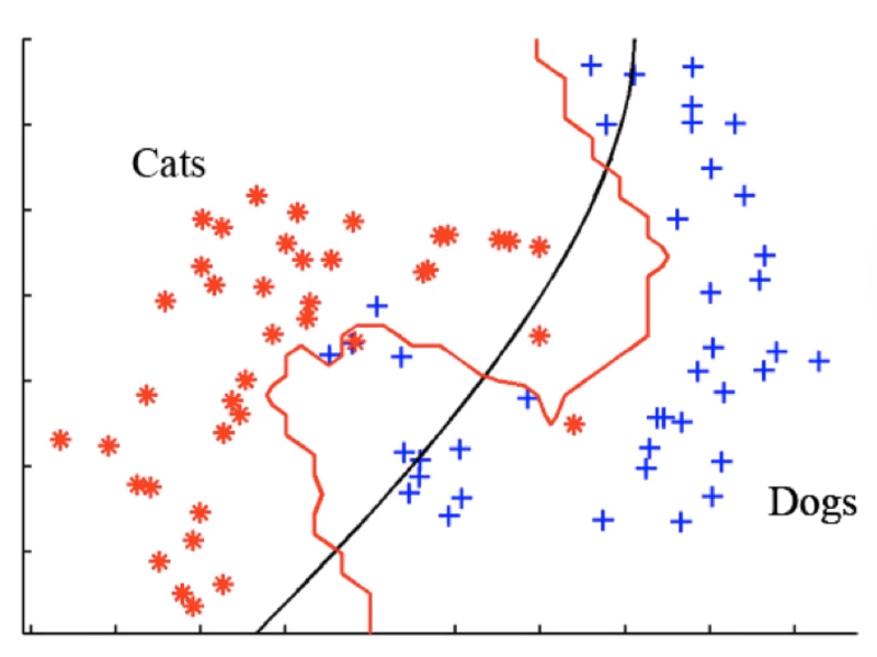
What is classification?
The classification consists of finding, through machine learning, a model or function that describes different data classes. The purpose of classification is to automatically label new instances of the database with a particular category by applying the model or function learned during training. This model is based on the value of the attributes of the training instances.
There are several classifiers available: KNN, Naive Bayes, Decision Trees… Classification can be used in several types of problems, such as:
- SPAM detection
- Automatic organization of emails by categorization
- Page ID with adult content
- Detection of expressions and feelings
Naive Bayes Classifier
The Classifier Naive Bayes is a probabilistic classifier based on applying the Bayes Theorem, with hypotheses of independence between attributes. In simple terms, the classifier Naive Bayes assumes that the presence or absence of a particular characteristic is not related to the presence or absence of any other element, taking into account the class’s target variable.
He is naive because he considers that each variable has independent participation, which does not always happen in practice.
For example, fruit can be considered an apple if red, round, and about 7 cm in diameter. A Naive Bayes classifier considers that each attribute contributes independently to the probability that this fruit is an apple, regardless of the presence or absence of other characteristics.
The Naive Bayes model is easy to build and particularly useful for large data sets. In addition to being simple, Naive Bayes is known to be superior to other highly sophisticated classification methods — in various classification problems, and we can achieve better results with Naive Bayes than with Artificial Neural Networks.
Naive Bayes Applications
There is no better Machine Learning algorithm than the other by itself. Each algorithm has advantages and disadvantages. The algorithm’s performance will be directly related to the business problem we are trying to solve and about our data set.
Naive Bayes can present a performance in neural networks for a given problem, while the Neural Networks have adequate performance for another issue. The important thing is to learn as much as possible about machine learning algorithms to try them out and achieve the best possible result.
• Multi-classes forecast
Fairly common use are multi-class predictions, i.e., when we have more than two classes that we must predict. For example, if we are trying to predict sentiment analysis, we need to expect whether a particular user is neutral, negative, positive, or any other feeling; in this case, we have few classes, and the Naive Bayes can be used for these situations.
• Text classification, spam filtering, and sentiment analysis
We can apply Naive Bayes to all three. Naive Bayes achieves excellent performance in many situations, especially when the data volume is not very large.
• Real-Time Predictions
When we need to collect real-time data from Twitter, Facebook, or any other data source and apply real-time classification, Naive Bayes performs well. It uses probabilistic calculations quickly compared to different algorithms.
So, if we have to use real-time online ranking, Naive Bayes is an excellent option.
• Recommendation System
When we have to find patterns in the data and from that, make recommendations for new users.
Naive Bayes at Scikit-learn
There are three types of Naive Bayes models in python’s Scikit-learn library. We have the algorithms:
1. Gaussian
The Gaussian algorithm considers the data to be in a normal distribution. If the data is already normalized, we can apply the Gaussian algorithm to The Naive Bayes.
2. Multinomial
This algorithm is used for discrete counts. If we have a text sorting problem, it would be necessary to count how often a word occurs in a document — from a statistical perspective; this problem would be the number of times an X value is observed during n attempts. For this, we can use the classifier Naive Bayes Multinomial.
3. Bernoulli
The Bernoulli Binomial model is helpful if the data vectors are binary, i.e., 0 and 1. An application would be to build a template for the classification of text. We want to know whether or not words occur in the document, i.e., 1 (the word occurs) 0 (the word does not appear), as this is typically a binary Bernoulli classification.
Probability Theory
To understand Bayes’ theorem, we need to take a step back and understand the theory of probability and what conditional probability is about.
Probability is the study of experiments that present results that cannot predict even under very similar conditions.
We studied probability intending to predict the possibilities of occurrence of a given situation or fact. Therefore, we studied probability to try to indicate the likelihood of an event occurring.
• Random Experiment
An experiment is considered random when its occurrences may present different results. An example of this happens when we flip a coin with distinct faces, one face and one crown. This release is unpredictable, as there is no way to know which face will be up.
• Sample Space
The sample space (S) determines the possible possibilities of results. In the case of the toss of a coin, the set of sample space is given by: S = {heads, tails} because they are the only two possible answers to this random experiment. Depending on the type of experiment, we can have a vast sample space.
• Event
The probability of the occurrence of a fact or situation is called an event. Therefore, when we launch a coin, we are establishing the occurrence of the event. We then have that any subset of the sample space should be considered an event. An example can happen when we flip a coin three times and get as a result of the event the following set: E = {heads, tails, heads}
• Probability Ratio
The probability ratio is given by the possibilities of an event occurring, taking into account its sample space. This ratio, which is a fraction, is equal to the number of event elements (numerator) over the number of features in the sample space (denominator).
This is the basis of probability theory. We have some variations in some forms that extend the concept of probability. We still have some general rules of probability based on the fact that probability is a value between 0 and 1 and is generally used in applying the Bayes theorem. To understand the Bayes theorem, we need to understand the concept of the conditional probability of simultaneous events.
Conditional Probability
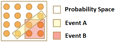
Conditional probability is the basic concept behind Bayes’ theorem. Below we have the space of possibilities of white background within the square, we still have event A which is the area with yellow background, and we have event B, which is the pink background square. Therefore, we have a total of possibilities and the occurrence of 2 events, and we can calculate the probability corresponding to a single event:
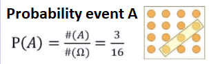
Above, we have 3 possibilities out of 16. Based on this, we can find probability A, an isolated event:
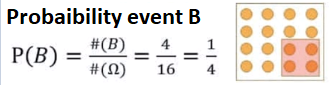
Just as we can try to find the probability of B, which is another isolated event, for this case, we have a chance of 25%.
Here we have the calculation of the individual probability of each event, but what we actually want is a conditional probability, that is, the occurrence of A given the occurrence of B and vice versa. Therefore, we are considering the likelihood of an event, given the occurrence of another event.
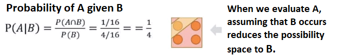
Calculating the conditional probability, we can see that the formula changes a little. We have P of A given B, i.e., Probability of A given the Occurrence of B — we break the procedure into two parts. At the top, we have the probability of A given B, divided by the individual probability of B.
When looking at the figure, we clearly have that the probability of A and B (intersection) is 1/16, and we still have the possibility of event B, which is 4/16.
We can do the opposite. Calculate the probability of B given the occurrence of A.
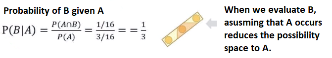
In many situations, to find the probability of an event, we have to consider the occurrence of another event, present in various scenarios in real life. Therefore, we saw the relationship between a conditional probability and its inverse probability, in other words, the likelihood of a hypothesis given the observation of evidence and the probability of the evidence presented by the hypothesis.
Bayes’ theorem represents one of the first attempts to model statistical inference to prove God’s existence mathematically. To achieve this goal, Bayes developed this theorem that became one of the bases of statistics.
Bayes Rules
The Bayes rule shows how to change odds a priori, considering new evidence to obtain a posteriori probability.

Above, we have the Bayes rule formula, with the a priori probabilities of P(x) and P(c), and we also have the probabilities a posteriori P(c|x) conditional to x and P(x|c) x conditional to c.
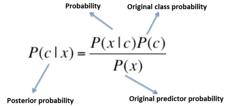
Bayes’ theorem provides a way to calculate the posterior probability, i.e., the posterior probability. Considering Bayes’s theorem formula, we have:
- P (c|x) is the later probability of the class (c, target) given the predictor (x, attributes).
- P © is the original probability of the class).
- P (x|c) is the probability of the predictor given the class.
- P (x) is the original probability of the predictor.
What the algorithm does in practice is learn these probabilities. During training, the algorithm will learn the chances to make up the formula and, in the end, present the likelihood of a given data point belonging to one of the classes for which we perform the training.
How does Bayes’s theorem work?
In probability theory, Bayes’ theorem shows the relationship between conditional probability and its inverse. Here we have a set of training data on “Weather” and the corresponding target variable “Play,” that is, according to the weather, what is the probability of a player playing sport or not.
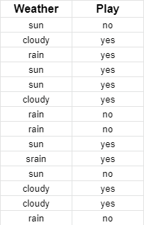
We have two independent events: climate and playing sports. Therefore, we need to sort whether athletes will play or not based on weather conditions. One event is conditioned to another; we use conditional probability to build Bayes’s theorem that considers conditional probability and its inverse. First, we must convert the dataset into a frequency table:
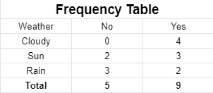
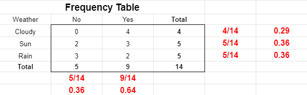
Then create probability tables to find the probabilities of each occurrence and each combination, that is, the total occurrences of an event divided by the entire possibilities.
Each class in the training set has its probability calculated. Most of the time, we work with only two categories, such as:
- whether or not a consumer purchases a product based on demographic characteristics
- whether or not a player will practice a sport given the weather condition
The calculation is done by dividing the number of instances of a given class by the number of cases in the training set.
Finally, we used the Bayes theorem equation to calculate the posterior probability for each class. The class with the highest posterior probability is the result of the prediction.

1st question: players will play sport if the fear is sunny. Is that statement correct? The first step is to find the odds we need to answer that question.
- P (Yes|Sun) = P (Sun|Yes) * P (Yes) / P (Sun)
Translating a Problem into Bayes’ Theorem
We have the first probability of (Yes| Sun), i.e., play, given that the day is sunny. Then we find its reverse, where we have the likelihood of a sunny day given the player practicing the sport P(Sun| Yes) and multiply by the probability of occurrence P(Yes) and divide by the possibility of making sun P(Sun).
Soon we will have to:
- P (Sun| Yes) = 3/9 = 0.33
- P (Sun) = 5/14 = 0.36
- P (Yes) = 9/14 = 0.64
And replace in the formula:
P (Yes|Sun) = P (Sun|Yes) * P (Yes) / P (Sun) = 0.33 * 0.64 / 0.36 = 0.60
So we’ll have a value of 0.60. As this is a relatively high probability, we can classify the result as Yes — players will practice sport if the weather is sunny.
Spam Classification with Naive Bayes in R
Using Naive Bayes is one of the most accessible activities in Machine Learning because the Naive Bayes algorithm has virtually no parameters, meaning there is practically nothing to configure in the algorithm regardless of the language we are using.
On the one hand, if it doesn’t have algorithm configuration parameters, it signals that we’ll have to do much more processing and deliver even better data to the algorithm. In some algorithms, as much as the data is not fully prepared, the algorithm achieves a resolution. With the Naive Bayes Algorithm, we don’t have this alternative; the data needs to be cut through a rich preprocessing, while the creation of the model will depend only on a line of code.
Filtering Spam Messages via SMS
For this example, we will use the SMS SPAM dataset. Naive Bayes is very useful for text sorting. Therefore, it works in conjunction with text mining tasks, mining text datasets, and then performing classifications.
Defining the Working Directory
getwd()
setwd(“documents/MachineLearning/naivebayes")
Load Packages
The tm package refers to text mining, wordcloud to build a word cloud, e1071, the Naive Bayes algorithm, and gmodels to create the confusion matrix.
install.packages(“slam”)
install.packages(“tm”)
install.packages(“SnowballC”)
install.packages(“wordcloud”)
install.packages(“gmodels”)
library(tm)
library(SnowballC)
library(wordcloud)
library(e1071)
library(gmodels)
Loading Data
data <- read.csv(“sms_spam.csv”, stringsAsFactors = FALSE)
Examining the structure of the data
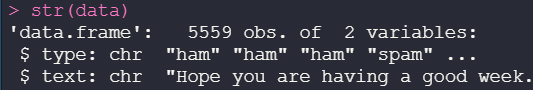
We have 5559 observations (rows) and two variables in the SPAM dataset.
str(data)
Building a Corpus
Corpus is a set of text documents, one of the essences of when working with text mining, that is, we convert our data set to a group of documents, and they will be treated in corpus form with the VCorpus function:
data_corpus <- VCorpus(VectorSource(data$text))
print(data_corpus)
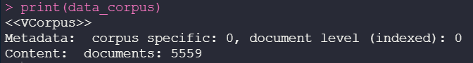
We can see that we have an object of the <<VCorpus>> that will allow us to perform differentiated treatments.
Examining the structure of the data
With Corpus objects, we can use the inspect function to analyze this dataset, that is, a summary about the dataset:
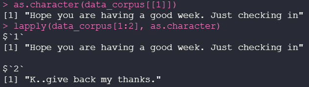
as.character(data_corpus[[1]])
lapply(data_corpus[1:2], as.character)

Adjusting the structure
We adjust the structure to return as a character and use lapply as a repeating structure to apply the same function to each of the DataFrame records:
as.character(data_corpus[[1]])
lapply(data_corpus[1:2], as.character)
Corpus Cleansing with tm_map()
The function tm_map transformations on Corpora, that is, it makes transformations in the Corpus.
?tm_map
data_corpus_clean <- tm_map(data_corpus, content_transformer(tolower))
In this case, we will use tolower to convert all characters to lowercase.
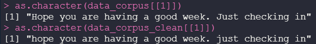
Differences between the initial Corpus and the Corpus after cleaning
as.character(data_corpus[[1]])
as.character(data_corpus_clean[[1]])
Other cleaning steps
The function tm_map transformations on Corpora, that is, it makes transformations in the Corpus.
data_corpus_clean <- tm_map(data_corpus_clean, removeNumbers)
data_corpus_clean <- tm_map(data_corpus_clean, removeWords, stopwords())
data_corpus_clean <- tm_map(daa_corpus_clean, removePunctuation)
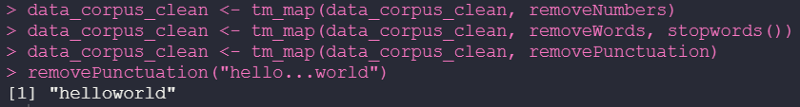
Creating a function to replace rather than removing punctuation
replacePunctuation <- function(x) { gsub(“[[:punct:]]+”, “ “, x) }
replacePunctuation(“hello…world”)
When we remove the score, we end up turning two words into a single word! Therefore, we will create a function to override rather than remove the score. We will replace the (…) with the space between words:
replacePunctuation <- function(x) { gsub(“[[:punct:]]+”, “ “, x) }
replacePunctuation(“hello…world”)
That way, we can maintain the integrity of the text.
Word stemming
Here we treat very similar words representing the same thing, the same information, and only in different verbal times. This for the predictive model may make no difference, and therefore, we will treat all these words as if they represent the same information:
?wordStem
wordStem(c(“learn”, “learned”, “learning”, “learns”))

Applying Stem
Here we apply the tm_map with stemDocument, that is, used the rule and searched very similar words to synthesize:
data_corpus_clean <- tm_map(data_corpus_clean, stemDocument)
Eliminating white space
We can eliminate unnecessary blanks:
data_corpus_clean <- tm_map(data_corpus_clean, stripWhitespace)
Examining the final version of Corpus
lapply(data_corpus[1:3], as.character)
lapply(data_corpus_clean[1:3], as.character)
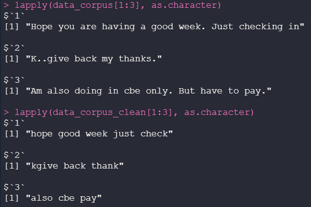
See that we replace the score, put everything in tiny, remove the stop words — standardized data.
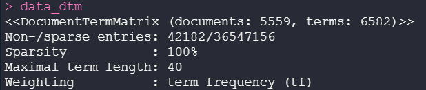
Solution 1- Creating a sparse document-term
Creating a simple, sparse matrix makes it easy for us to build graphs and a predictive model.
?DocumentTermMatrix
dados_dtm <- DocumentTermMatrix(dados_corpus_clean)
Solution 2 — creating a sparse document-term matrix direct from Corpus
data_dtm2 <- DocumentTermMatrix(data_corpus, control = list(tolower = TRUE, removeNumbers = TRUE, stopwords = TRUE, removePunctuation = TRUE, stemming = TRUE))
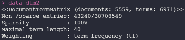
This second procedure considerably increased the number of terms from 6582 to 6971, which probably indicates that it could not remove some stop words — being the worst procedure applied among the three.
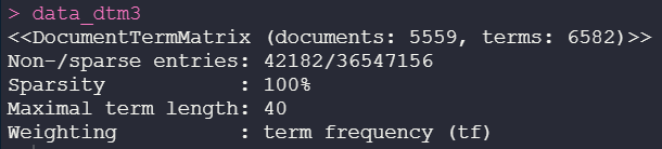
In this third sparse array, we now use a specific function to remove stop words:
Solution 3 — using custom stop words from the function
dados_dtm_train <- data_dtm[1:4169, ]
dados_dtm_test <- data_dtm[4170:5559, ]
Creating training and test datasets
We made a subset of the training data, and the remaining ones went to the test data:
dados_dtm_train <- data_dtm[1:4169, ]
dados_dtm_test <- data_dtm[4170:5559, ]
Labels (target variable)
We will do the same procedure with the labels, that is, with the target variable that is the factored type column:
dados_train_labels <- data[1:4169, ]$type
dados_test_labels <- data[4170:5559, ]$type
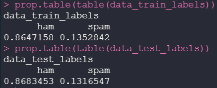
Checking if the spam ratio is similar
Here we compared the proportion of Spam and Ham with the prop.table function, this ratio should be very similar:
prop.table(table(data_train_labels))
prop.table(table(data_test_labels))
Word Cloud
Let’s unify everything in a word cloud with the function itself and return an image where the most frequent words are more prominent.
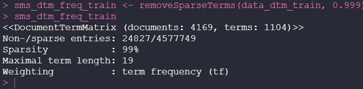
sms_dtm_freq_train <- removeSparseTerms(data_dtm_train, 0.999)
sms_dtm_freq_train
Data frequency
We will collect from the dataset the words that appear most frequently. In practice, we will be decreasing our sparse matrix by containing only the most frequent words:
findFreqTerms(data_dtm_train, 5)
Features indicator for frequent words
We can use the findFreqTerms function to find the words that appear most frequently:
sms_freq_words <- findFreqTerms(data_dtm_train, 5)
str(sms_freq_words)

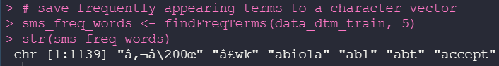
Save frequently-appearing terms to a character vector
We use these most frequent words to generate a new dataset. We will put the result of findFreqTerms in the sms_freq_words:
sms_freq_words <- findFreqTerms(data_dtm_train, 5)
str(sms_freq_words)
Creating subsets only with more frequent words
Rebuilding the training and test dataset with the most frequent words to deliver to the predictive model:
ms_dtm_freq_train <- data_dtm_train[ , sms_freq_words]
sms_dtm_freq_test <- data_dtm_test[ , sms_freq_words]
Converting to factor
Here we convert the count to factor and apply this conversion to our training and test datasets (adequately cleaned and organized):
convert_counts <- function(x) {
  print(x)
  x <- ifelse(x > 0, "Yes", "No")
}
Converting counts to training and test data columns with apply()
sms_train <- apply(sms_dtm_freq_train, MARGIN = 2, convert_counts)
sms_test <- apply(sms_dtm_freq_test, MARGIN = 2, convert_counts)
Building Naive Bayes model
Finally, we started the construction of the model.
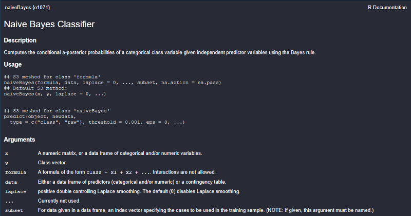
?naiveBayes
Training the Naive Bayes model
nb_classifier <- naiveBayes(sms_train, data_train_labels)

We call the naiveBayes function and pass the training and test datasets to the nb_classifier.
Evaluating model 31
We evaluate the predictive model nb_classifier by presenting it with a new set of test data, that is so that it can make predictions whether or not we have SPAM in the collection:
sms_test_pred <- predict(nb_classifier, sms_test)
Confusion Matrix
We built Confusion Matrix so we can compare and see the result of our model:
CrossTable(sms_test_pred,
 dados_test_labels,
 prop.chisq = FALSE,
 prop.t = FALSE,
 prop.r = FALSE,
 dnn = c(‘Predicted’, ‘Observed’))
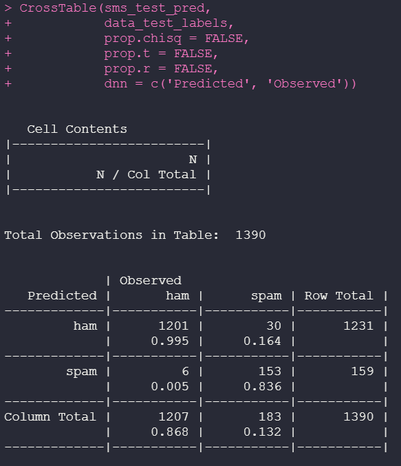
We have the values predicted against those observed. The predicted value is what the model predicted, and the observed is the historical data that we present to the model. The classifier performed with an excellent level of accuracy.
Improving model performance by applying Laplace smoothing
A common problem when working with Naive Bayes is the problem of frequency 0. We are working with text sorting! Some words may have gone to the test suite, but they may not have gone to the training set, interfering with learning the algorithm.
To mitigate the frequency problem 0, we can apply the Laplace estimator, smoothing; when the model does not find a word instead of putting a probability 0, it will put counter 1.
nb_classifier_v2 <- naiveBayes(sms_train, data_train_labels, laplace = 1)
Evaluating model
sms_test_pred2 <- predict(nb_classifier_v2, sms_test)
nb_classifier_v2 <- naiveBayes(sms_train, data_train_labels, laplace = 1)
Confusion Matrix
CrossTable(sms_test_pred2,
 dados_test_labels,
 prop.chisq = FALSE,
 prop.t = FALSE,
 prop.r = FALSE,
 dnn = c(‘Predicted’, ‘Observed"))
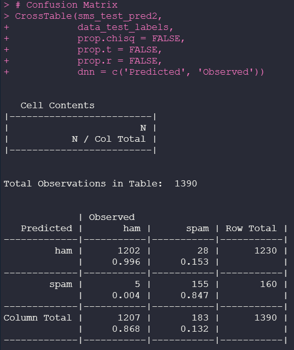
We’ve managed to reduce the number of errors! Before, we had 30 errors where the observed value was SPAM, and the predicted value was HAM; now, we have 28 applying only the Laplace method. Therefore, we increased the true positives that used to be from 0.995 to 0.996 and decreased the false positive rate.
Note: To make new predictions with the trained model, generate a new mass of data and use the predict() function.
Naive Bayes is extremely powerful and is compared in performance to some sophisticated machine learning models when working with text classification — the secret lies in the data processing.
And there we have it. I hope you have found this helpful. Thank you for reading. ?
A Detailed Naive Bayes Spam Filter in R was originally published in Level Up Coding on Medium, where people are continuing the conversation by highlighting and responding to this story.
This content originally appeared on Level Up Coding - Medium and was authored by Anello
Anello | Sciencx (2021-06-15T03:35:53+00:00) A Detailed Naive Bayes Spam Filter in R. Retrieved from https://www.scien.cx/2021/06/15/a-detailed-naive-bayes-spam-filter-in-r/
Please log in to upload a file.
There are no updates yet.
Click the Upload button above to add an update.