
This content originally appeared on Bits and Pieces - Medium and was authored by Stephen Jose
Part 1: Everything a programmer needs to know about time complexity, from zero to hero.
When starting time complexity, most get confused with time complexity as the running time (clock time) of an algorithm. The running time of the algorithm is how long it takes for the computer to run the lines of code to completion and the running time it depends on.
- The speed of the computer (Hardware).
- The programming language used (Java, C++, Python).
- The compiler that translates our code into machine code (Clang, GCC, Min GW).
Considering the running time (clock time) of an algorithm is not an efficient way of calculating the time complexity of an algorithm. This is because each computer will have different speeds and each user has their own preferences on which programming language they use. For this reason, we need a common way to calculate the efficiency(time complexity) of our algorithm.
Then we will be able to compare it with other similar algorithms. Now we will look into a more standard way of calculating the efficiency(time complexity) of algorithms using various asymptotic notations.
Time complexity is a function that describes the amount of time required to run an algorithm, as input size of the algorithm increases.
In the above definition note, “time” doesn’t mean wall clock time, it basically means how number of operations performed by the algorithm grows as the input size increases. Operations are the steps performed by an algorithm for the given input.
Calculating time complexity by the growth of the algorithm is the most reliable way of calculating the efficiency of an algorithm. It is independent of hardware, programming language, or compilers used. By operations in an algorithm we mean.
- Assigning values to variables.
- Making comparisons.
- Executing arithmetic operations.
- Accessing objects from memory.
We use this abstract method of measuring, time complexity in terms of growth. That is how the number of operations performed by the algorithm increases as the input size increases.
Calculating Time complexity of Linear Search
Linear search is the simplest algorithm to search for an element x in an array. It examines each value in an array and compares it to element that needs to be searched until it finds a match, starting from the beginning. The search is finished and terminated once the target element gets located.
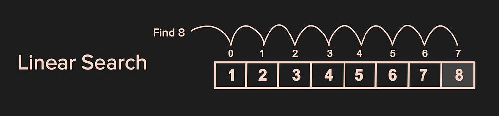
In the example above, the array has 8 values 1,2,3,4,5,6,7,8. Suppose we want to search for an element 8, the algorithm compares 8 with each element of the array until it finds a match. Once it finds the match the index of 8 which is7 is returned, else suppose if 9 was not in the array then -1 will be returned.
Code Implementation of Linear Search
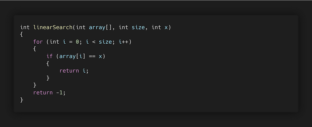
The above code snippet is a function for linear search, which takes in an array, the size of the array and the element to be searched x.
Time Complexity Analysis
While performing a linear search algorithm, you will be faced with three different complexities.
They are:
- Best Case
- Worst Case
- Average Case
Best Case
If the element that is searched is found in the first position of the array then, in that case, the search will end with a single successful comparison. In the best-case scenario, the algorithm performs O(1) operations. O (Big-Oh is a notation used to represent time complexity).
Worst Case
If the element that is searched is found in the last position of the array or not found at all. Then the search executes for n comparisons. Thus, in a worst-case scenario, the algorithm performs O(n) operations.
Average Case
If the element to be searched is in the middle of the array, then the average number of comparisons is n/2. Thus, in the average case scenario, it performs O(n). We ignore 1/2 constant, we will understand, why we ignore constants while learning Asymptotic Notation.
Calculating Time Complexity of Binary Search
A binary search is one of the most efficient searching algorithms, it searches an element in a given list of sorted elements. It reduces the size of the array to be searched by half at each step. Binary search makes fewer guesses compared to linear search. When binary search makes an incorrect guess, the array will be reduced to half its original size.
For example, if the array has 10 elements, then incorrect guess cuts the array down to 5 elements.

In the example above, we have an array with eight values1,2,3,4,5,6,7,8 and the element to be searched is 8.
- In the first step, the middle element of the array gets calculated by (0+7)/2=3, then it compares the middle element 4 with 8.
- If the search element 8 is greater than the middle element 4. Then the right half is searched.
- If the search element 8 is less than the middle element 4. Then the left half is searched.
- These steps get repeated until the search element 8is found or the condition L>H is met, which indicates the element was not found and -1 is returned.
Code Implementation of Binary Search
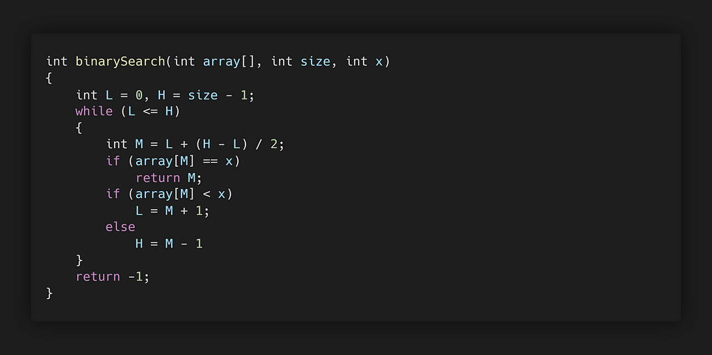
The above code snippet is a function for binary search, which takes in an array, size of the array, and the element to be searched x.
Note: To prevent integer overflow we use M=L+(H-L)/2 , formula to calculate the middle element, instead M=(H+L)/2.
Time Complexity of Binary Search
At each iteration, the array is divided by half its original size, so let's say the length of the array at the beginning of the iteration is N, then the complexity at each iteration is calculated as
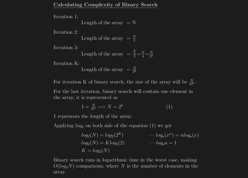
Time Complexity Analysis of Binary Search
Best Case
The best time complexity of the binary search is when the search element is in the middle of the array. Then the number of comparisons would be O(1).
Average Case
The average time complexity is when the search element is in the array and the time complexity would be O(logN).
Worst Case
The worst case occurs when the search element is not in the array or is found at the last iteration of the binary search. The time complexity would be O(logN).
Comparison of Binary Search and Linear Search
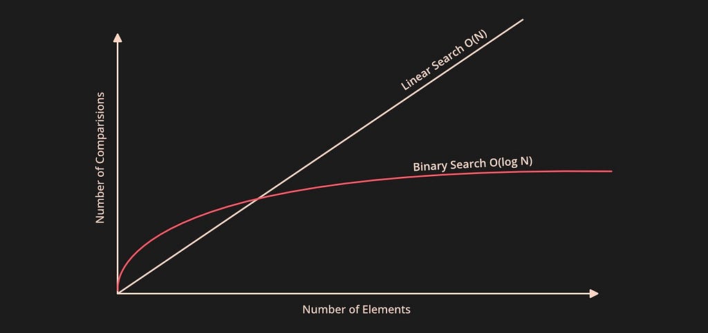
In the graph above, we can observe that when the array size is large enough the time complexity of the binary search is considerably better than the linear search. Cause of logarithmic time complexity of the binary search, whereas linear search, has linear time complexity.
Both linear and binary search algorithms can be useful depending upon the application. When the array elements are sorted, the binary search is preferred for a quick search. Linear search performs with the help of sequential access by making n comparisons for n number of elements in the array.
Binary search algorithms are known to search by accessing the data randomly, taking only logn comparison for n elements in the array.
Asymptotic Notations
Asymptotic notation is one of the most efficient ways to calculate the time complexity of an algorithm.
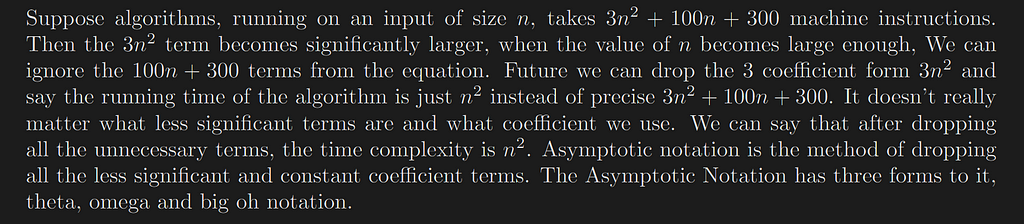
Suppose algorithms, running on an input of size n, takes 3 n²+100 n+300 machine instructions. Then the 3 n² term becomes significantly larger, when the value of n becomes large enough, We can ignore the 100 n+300 terms from the equation.
Further we can drop the 3 coefficient form 3 n² and say the running time of the algorithm is just n² instead of precise 3 n²+100 n+300. It doesn’t really matter what less significant terms are and what coefficient we use. We can say that after dropping all the unnecessary terms, the time complexity is n². Asymptotic notation is the method of dropping all the less significant and constant coefficient terms.
The Asymptotic Notation has three forms to it, big theta, big omega and big oh notation.
A short definition of asymptotic notation
Asymptotic Notations are mathematical tools used to represent the complexities of an algorithm.
There are three forms of asymptotic notations
- Big O (Big-Oh)
- Big Ω (Big-Omega)
- Big Θ (Big-Theta)
Big-Oh Notation
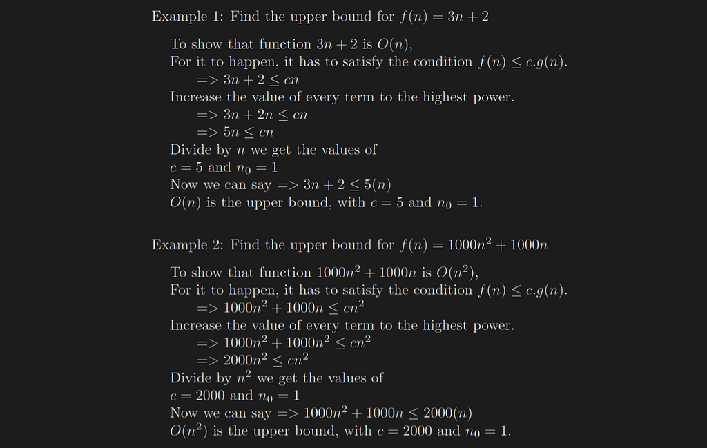
Big Oh is an Asymptotic Notation for the worst-case scenario, which is also the ceiling of growth for a given function. It provides us with what is called an asymptotic upper bound for the growth, of an algorithm.
The Mathematical Definition of Big-Oh
f(n) ∈ O(g(n)) if and only if there exist some positive constant c and some non-negative integer n₀ such that, f(n) ≤ c g(n) for all n ≥ n₀, n₀ ≥ 1 and c>0.

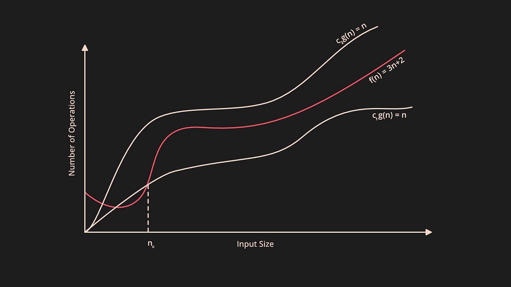
The above definition says in the worst case, let the function f(n) be your algorithm's runtime, and g(n) be an arbitrary time complexity you are trying to relate to your algorithm. Then O(g(n)) says that the function f(n) never grows faster than g(n) that is f(n)<=g(n)and g(n) is the maximum number of steps that the algorithm can attain.
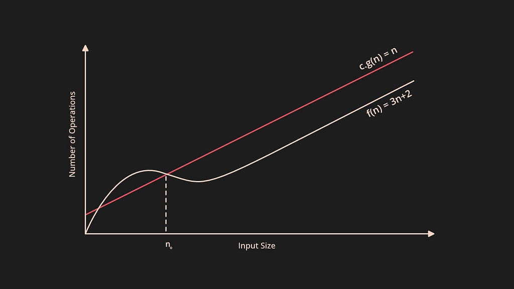
In the above graph, the c.g(n)is a function that gives the maximum runtime(upper bound) and f(n) is the algorithm’s runtime.
Examples of Big-O Notation
Big-Omega Notation
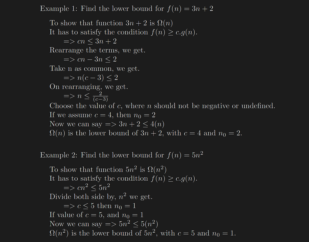
Big Omega is an Asymptotic Notation for the best-case scenario. Which is the floor of growth for a given function. It provides us with what is called an asymptotic lower bound for the growth rate of an algorithm.
The Mathematical Definition of Big-Omega
f(n) ∈ Ω(g(n)) if and only if there exist some positive constant c and some non-negative integer n₀ such that, f(n) ≥ c g(n) for all n ≥ n₀, n₀ ≥ 1 and c>0.

The above definition says in the best case, let the function f(n)be your algorithm’s runtime and g(n) be an arbitrary time complexity you are trying to relate to your algorithm. Then Ω(g(n)) says that the function g(n)never grows more than f(n)i.e. f(n)>=g(n), g(n)indicates the minimum number of steps that the algorithm will attain.

In the above graph, the c.g(n)is a function that gives the minimum runtime(lower bound) and f(n)is the algorithm’s runtime.
Examples of Big-Ω Notation
Big-Theta Notation
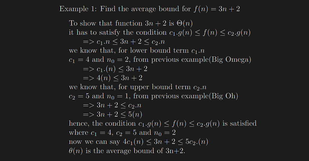
Big Theta is an Asymptotic Notation for the average case, which gives the average growth for a given function. Theta Notation is always between the lower bound and the upper bound. It provides us with what is called an asymptotic average bound for the growth rate of an algorithm. If the upper bound and lower bound of the function give the same result, then the Θ notation will also have the same rate of growth.
The Mathematical Definition of Big-Theta
f(n) ∈ Θ(g(n)) if and only if there exist some positive constant c₁ and c₂ some non-negative integer n₀ such that, c₁ g(n) ≤ f(n) ≤ c₂ g(n) for all n ≥ n₀, n₀ ≥ 1 and c>0.

The above definition says in the average case, let the function f(n)be your algorithm runtime and g(n)be an arbitrary time complexity you are trying to relate to your algorithm. Then Θ(g(n)) says that the function g(n)encloses the function f(n)from above and below using c1.g(n) and c2.g(n).
In the above graph, the c1.g(n)and c2.g(n)encloses the function f(n). This Θ notation gives the realistic time complexity of an algorithm.
Examples of Big-Θ Notation
Calculating the Time Complexity for the following Algorithms
We will determine the different time complexity of algorithms, in terms of big O notation, we will be using Big-O because it is the case that we should be concerned about. Algorithms are mostly tested for the worst-case scenario.
Example 1: Loops
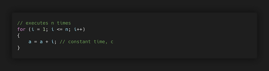
The running time of a loop is the multiple of, statements inside the loop by the number of iterations.
Total Time = constant c × n = c n = O(n)
Example 2: Nested Loops
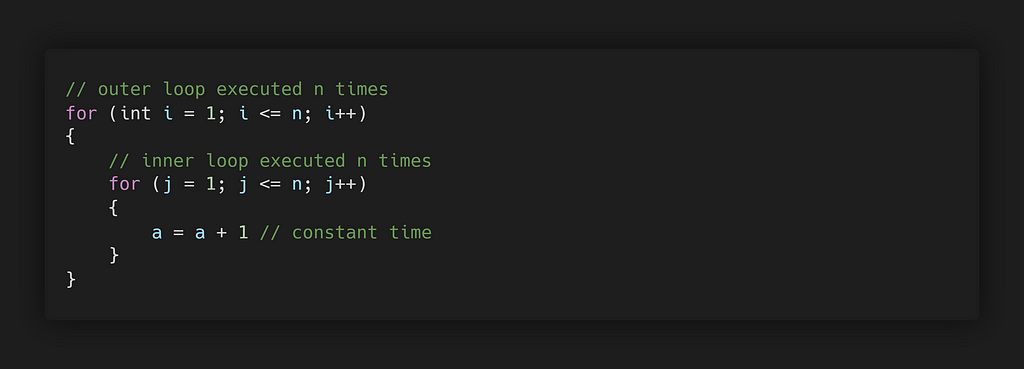
The total running time of this algorithm is the product of the sizes of all the loops.
Total Time = c × n × n = cn² = O(n²)
Example 3: Consecutive Statements
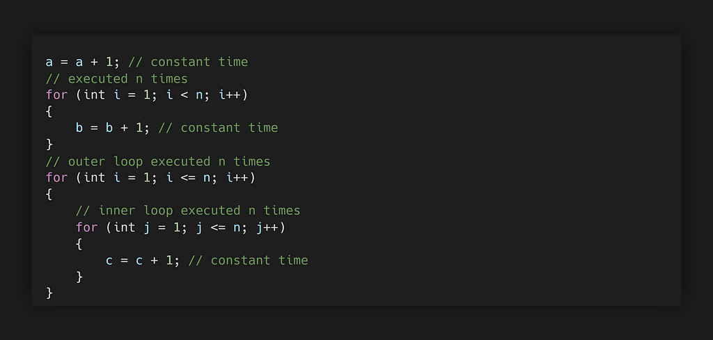
The total running time of this algorithm is the sum of all the time complexities of each statement of the algorithm.
Total Time = c₀ + c₁n + c₂n² = O(n²)
Example 4: Logarithmic Complexity
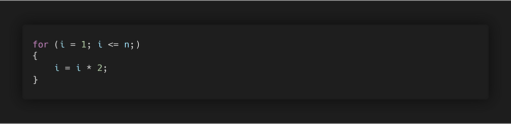
If we observe the value of iit is doubling on every iteration i=1,2,4,8.. , and the original problem is cut by a fraction (1/2)on each iteration, the complexity of this kind is of log time.
Total Time = O(logn)
Part 2
To learn more about asymptotic notations refer the Part 2 of this article.
- Asymptotic Notation using Limits.
- Time Complexity of Recursive Algorithms.
- Time Complexity of Divide and Conquer Algorithms.
- Masters Theorem.
- Akra-Bazzi Method.
Build composable web applications
Don’t build web monoliths. Use Bit to create and compose decoupled software components — in your favorite frameworks like React or Node. Build scalable and modular applications with a powerful and enjoyable dev experience.
Bring your team to Bit Cloud to host and collaborate on components together, and speed up, scale, and standardize development as a team. Try composable frontends with a Design System or Micro Frontends, or explore the composable backend with serverside components.

Learn More
- How We Build Micro Frontends
- How we Build a Component Design System
- The Composable Enterprise: A Guide
- 7 Tools for Faster Frontend Development in 2022
How to Calculate Time Complexity from Scratch was originally published in Bits and Pieces on Medium, where people are continuing the conversation by highlighting and responding to this story.
This content originally appeared on Bits and Pieces - Medium and was authored by Stephen Jose
Stephen Jose | Sciencx (2022-04-06T08:35:38+00:00) How to Calculate Time Complexity from Scratch. Retrieved from https://www.scien.cx/2022/04/06/how-to-calculate-time-complexity-from-scratch/
Please log in to upload a file.
There are no updates yet.
Click the Upload button above to add an update.