
This content originally appeared on DEV Community 👩💻👨💻 and was authored by Alexey Timin
A popular approach for conditional monitoring of mechanical machines is to embed vibration sensors into a machine and start "listening" to it. The data from the sensors must be stored somewhere. So, the more efficient we compress them, the longer history we can keep. When we deal with sensors we always have noise from them, and when a machine is stopped we have only noise which wastes our storage space. WaveletBuffer was developed to solve this problem by using the wavelet transformation and efficient compression of denoised data. However, a user must know many settings to use it efficiently. In this tutorial, you will learn how to find denoising parameters to get rid of white noise in your data.
Basics
For an educational purpose, I brought two samples from a vibration sensor which is maintained on a real machine. You can find them in the directory docs/tutorials. buffer_signal.bin contains a second of the signal when the machine is working. buffer_no_signal.bin has only noise because the machine is stopped. Both files are serialized buffer without any denoising, so they have equal sizes but different amount of the information!
We need to separate white noise and information, so we need the sample with the working machine. Let's deserialize it:
from wavelet_buffer import WaveletBuffer, denoise
import numpy as np
import matplotlib.pyplot as plt

blob = b""
with open("buffer_signal.bin", "rb") as f:
    blob = f.read()

print(f"Initial size {len(blob)/ 1000} kB")
buffer = WaveletBuffer.parse(blob)
print(buffer)
Output:
Initial size 194.918 kB
WaveletBuffer<signal_number=1, signal_shape=(48199), decomposition_steps=9, wavelet_type=WaveletType.DB3>
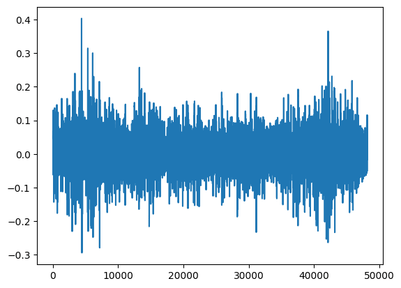
You can see that the signal has about 48000 points and the size of the file is about 200kB. Let's have a look at the signal inside:
signal = buffer.compose()

plt.plot(signal)
plt.show()

Looks noisy, right? When we've restored the original signal, we can use WaveletBuffer to denoise it. We use some random threshold for the demonstration. Later we learn how to find the optimal parameter. When we pass denoise.Threshold(a=0, b=0.04) in WaveletBuffer.decompose method it set to 0 all values in hi-frequency subbands which less than a*x+b where x is a decomposition step of the current subband.
buffer.decompose(
    signal, denoise.Threshold(a=0, b=0.04)
)  # this a*x + 0.04 where x is a decomposition step
denoised = buffer.compose()
plt.plot(denoised)
plt.show()

Information Loosing Detection
The denoised signal looks the same, but we actually don't know if we removed only the noise, or we removed some part of the signal. To figure out it, we can take the difference between the denoised and original signals and check if it has some information or only noise. It has some information and means we deleted with denoising.
err = denoised - signal
plt.plot(err)
plt.show()

To check if the difference (err) has something more than only noise we can find autocorrelation of error and test if all the values lie within [-1.96/sqrt(n), 1.96.sqrt(n)] where n is the size of sample. For more detail, see here.
def autocorr(x):
    result = np.correlate(x, x, mode="full")
    return result[int(len(result) / 2) :]


def test(corr: np.ndarray):
    thr = 1.96 / np.sqrt(len(corr))
    tests = np.where(np.abs(corr) <= thr, 0, 1)
    return tests.sum() == 0


corr = autocorr(err)
print(test(corr))
Output
False
Optimal Denoise Parameters
You can see that for denoise.Threshold(0, 0.04) we removed something important from our signal. However, the desnoised signal looked the same. To find the optimal threshold, we can start from 0 and increasing the threshold with a little step until we fail the test:
threshold = 0
step = 0.0001
for x in range(1000):
    threshold = step * x
    buffer.decompose(signal, denoise.Threshold(0, threshold))
    err = buffer.compose() - signal
    corr = autocorr(err)
    if not test(corr):
        threshold = threshold - step
        print(f"Optimal threshold: {threshold}")
        break
Output:
Optimal threshold: 0.0017000000000000001
You see that the threshold way less than our initial assumption. Let's check the size of serialized signal:
buffer.decompose(signal, denoise.Threshold(0, threshold))
print(f"Compression size: {len(buffer.serialize(compression_level=16)) / 1000} kB")

signal = buffer.compose()

plt.plot(signal)
plt.show()
Output:
Compression size: 58.528 kB
Looks like it got 3.5 times smaller after the demonising. However, the most interesting thing is compression of the sample when the machine was stopped:
blob = b""
with open("buffer_no_signal.bin", "rb") as f:
    blob = f.read()

buffer = WaveletBuffer.parse(blob)
buffer.decompose(buffer.compose(), denoise.Threshold(0, threshold))
signal = buffer.compose()

print(
    f"Compression (onlynoise) size: {len(buffer.serialize(compression_level=16)) / 1000} kB"
)

plt.plot(signal)
plt.show()
Output:
Compression (onlynoise) size: 0.41 kB

The compressed size is 500 times smaller now, because we don't have valuable information in the sample.
Conclusion
WaveletBuffer provides a pipeline wavelet transormation -> denoising -> compression which is useful for efficient compression of height frequency time series data. This approach has an additional advantage for data sources which don't provide valuable information all the time but are requested continuously.
References:
- White Noise Model - Time Series Analysis, Regression and Forecasting
- WaveletBuffer - A universal C++ compression library based on wavelet transformation
- WaveletBuffer for Python - Python bindings for WaveletBuffer
This content originally appeared on DEV Community 👩💻👨💻 and was authored by Alexey Timin
Alexey Timin | Sciencx (2022-09-12T15:34:32+00:00) Denoising time series data by using wavelet transformation. Retrieved from https://www.scien.cx/2022/09/12/denoising-time-series-data-by-using-wavelet-transformation/
Please log in to upload a file.
There are no updates yet.
Click the Upload button above to add an update.