How We Turned the iPhone into a Laboratory Microscope with AI and BLE

This content originally appeared on HackerNoon and was authored by Amin Benarieb

Introduction

In this article, I want to share my experience developing an iOS application for a robotic microscope with AI-based blood cell recognition — how it’s built, the challenges we had to tackle, the pitfalls we encountered, and how the iPhone can be used as a laboratory tool.

This is not yet another to-do list app with authentication or an application for applying filters to selfies — the focus here is on a video stream from the microscope’s eyepiece, neural networks, hardware interaction, Bluetooth-controlled slide movement, and all of this running directly on the iPhone. At the same time, I’ve tried not to delve into excessive technical detail, so the article remains accessible to a broader audience

A Few Words About the Product

Even with modern hematology analyzers, up to 15% of samples still require manual review under a microscope — especially when anomalies are found in the blood. Automated microscopy systems do exist, but they cost as much as an airplane wing, which is why most laboratories continue to examine blood smears manually. We’re doing it differently: our solution turns a standard laboratory microscope into a digital scanner with automated slide feeding and image capture — simple, affordable, and efficient. We’re developing it together with @ansaril3 and the team in celly.ai.

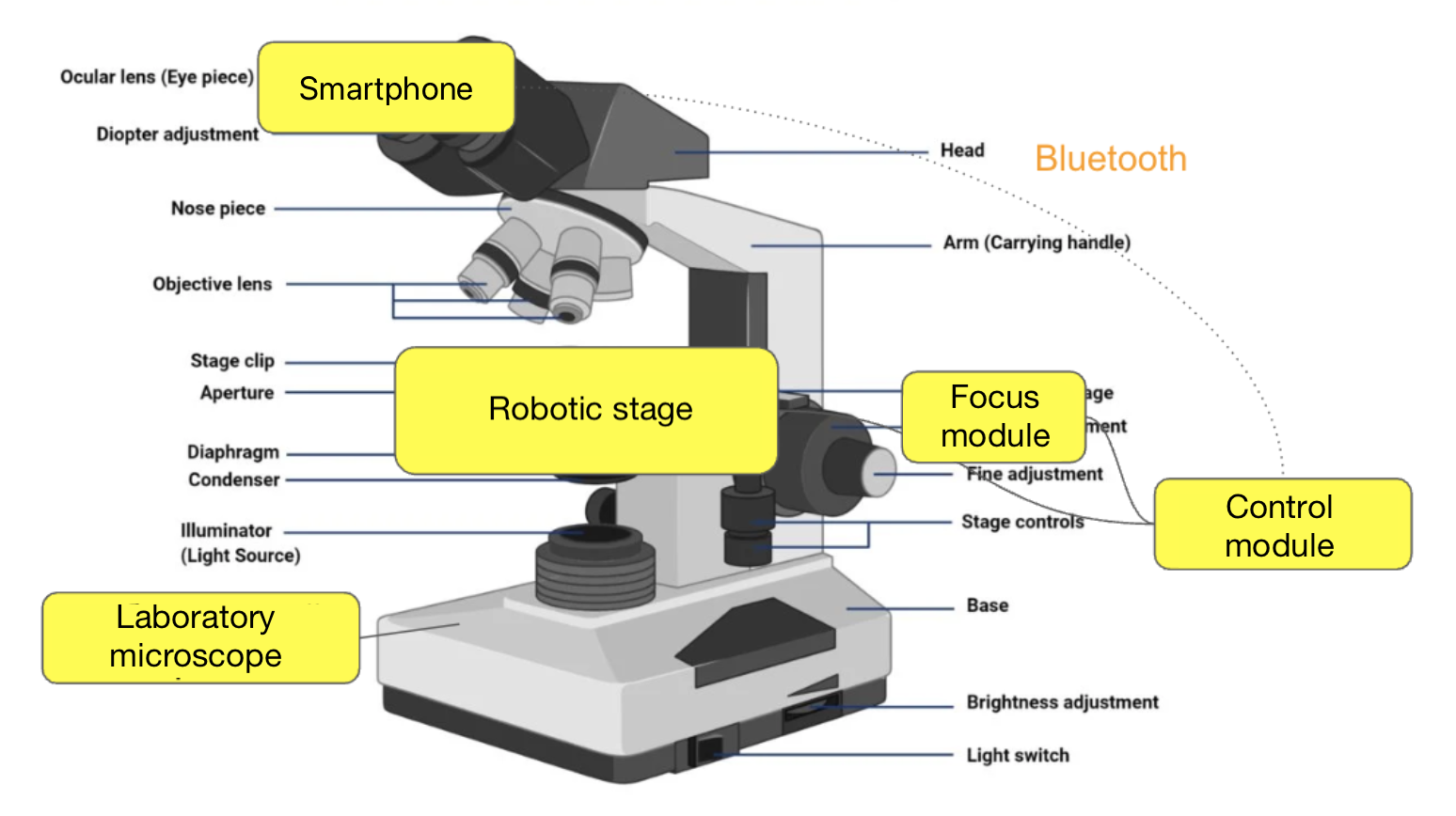
The kit connects to a standard laboratory microscope, transforming it into a digital scanner. Its hardware components include:

• iPhone — system control, cell analysis
• Lens adapter — connecting the smartphone to the microscope’s eyepiece
• Robotic stage — enables slide movement, focus control, and switching between samples

On the software side, the system consists of:

• a mobile application on the iPhone

• a controller on the stage

• a web portal/cloud

  

The mobile application performs the following tasks:

• processes the image stream from the camera, detects, classifies, and counts cells
• sends them to the web server along with other analysis artifacts
• controls the movement of the robotic stage, performing smear scanning according to a predefined algorithm
• and is also responsible for configuration and analysis initiation, camera parameter adjustments, viewing a brief analysis report, and other related tasks

The web portal is intended for viewing results, physician confirmation of the analysis, and report export. Below is a video showing how it all works together:

\

A Bit of Context About Hematological Diagnostics

The primary analysis we perform is blood smear microscopy. It’s a component of the Complete Blood Count (CBC), one of the most common and fundamental medical tests. Many people have undergone it and have seen similar tables in their results (source):

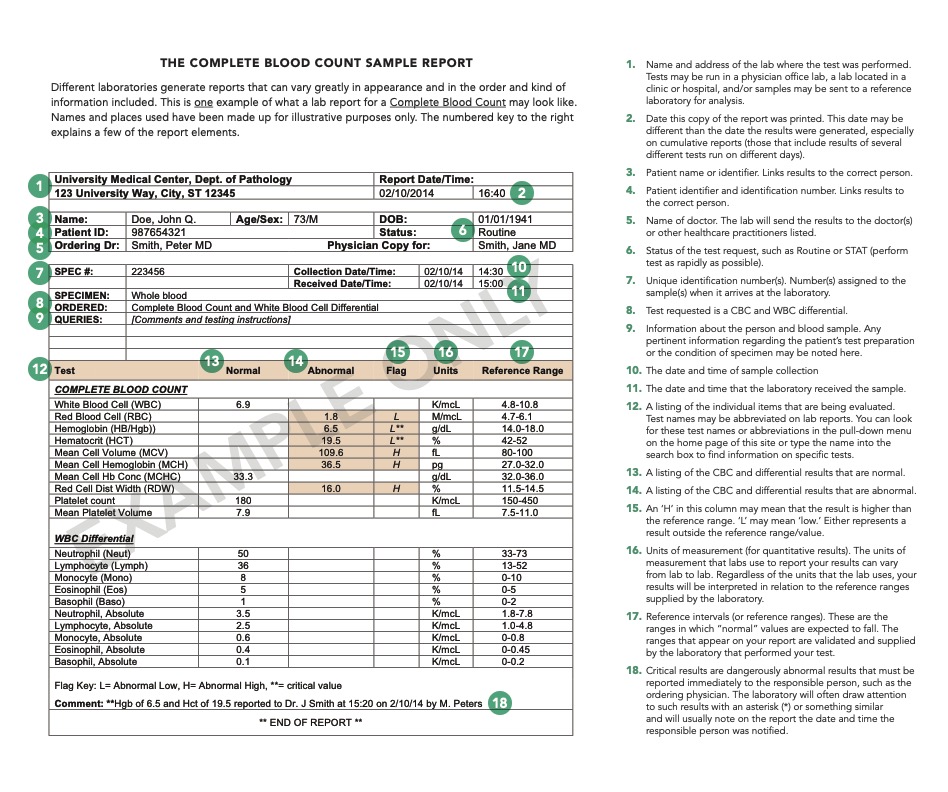
When performing a CBC, blood samples are processed through a hematology analyzer. If the device indicates a deviation from the norm, the sample undergoes microscopic examination.

This process looks as follows:

• a lab technician places a drop of blood onto a glass slide,

• stains it using the Romanowsky method (or similar alternatives<)¹ , fixes it,

• and examines the prepared smear under the microscope visually.

  

It’s precisely at this stage that one can:

• detect abnormal cell morphologies (such as immature neutrophils, atypical lymphocytes, blast cells),
• assess maturity, size, granularity, inclusions, and other parameters,
• and sometimes even make a preliminary diagnosis before obtaining PCR² or ELISA³   data.

But manual analysis is painful:

• it’s highly subjective,
• depends on the technician’s experience,
• humans are prone to fatigue and errors,
• and it doesn’t scale well.

Automated microscopy systems are excellent, but they’re expensive (starting from 60000$ and above), which is why more than 90% of laboratories still rely on the manual method!

We set ourselves the goal of creating an affordable microscope automation kit (within several hundred thousand rubles) that could be widely deployed in laboratories. And this is where the iPhone comes onto the stage.

[1] - A blood sample on the slide is treated with a special stain developed by Dmitry Leonidovich Romanowsky (1861–1921). This stain makes various components of blood cells more visible under the microscope, as they are stained in different colors

[2] - PCR (Polymerase Chain Reaction) makes it possible to detect even very small amounts of genetic material, such as viruses or bacteria, which is crucial for diagnosing infectious diseases. We remember this well from the COVID era

[3] - ELISA (Enzyme-Linked Immunosorbent Assay) is used when it’s important to detect the presence of specific proteins

What the iPhone Is Capable Of

When we talk about “AI on a smartphone,” most people picture things like camera filters, text autocomplete, or chatbots. But modern iPhones are mini-computers with dedicated neural modules capable of performing serious tasks — in our case, real-time blood cell analysis. Let’s look at three key components that make this possible:

• Graphics Processing Unit (GPU). Used for image operations: preprocessing, filtering, correction. For example: blur assessment, color correction, artifact removal, and other specific tasks related to graphics and image analysis.
• Neural Processing Unit (NPU / Neural Engine). Apple has been integrating the Neural Engine into its devices starting with the A11 chip (iPhone 8/X), and from the A12 (iPhone XR and newer), it’s already possible to perform over 5 trillion operations per second on the NPU (TOPS). At the time of writing, the latest A17 Pro and A18/A18 Pro chips are capable of 35 TOPS. This is used for inference of models for cell detection and classification, background assessment of the specimen, and similar tasks, freeing up the CPU/GPU.
• Central Processing Unit (CPU). Responsible for overall logic, control, configuration processing, serialization/deserialization, working with APIs and the file system — essentially everything that doesn’t fall under the previous two components.

We’ll be discussing this using the iPhone XR (A12 Bionic, 2018) as a sort of baseline, even though it’s already an older device. Even on this model, we were able to:

• process a 50fps video stream from the microscope camera,
• simultaneously perform CoreML inference (~15ms per frame),
• concurrently save data to disk and synchronize with the cloud,
• keep the temperature within acceptable limits (if throttling and task prioritization are carefully configured).

Nevertheless, the device could noticeably heat up and start slowing down. For instance, during the analysis of malaria smears, where it’s necessary to process over 100 cells in a single frame, thermal throttling would begin as early as the second or third smear — CPU frequency would drop, and interface lags and slowdowns would appear. Moreover, the close contact of the adapter against the device’s rear panel hinders heat dissipation

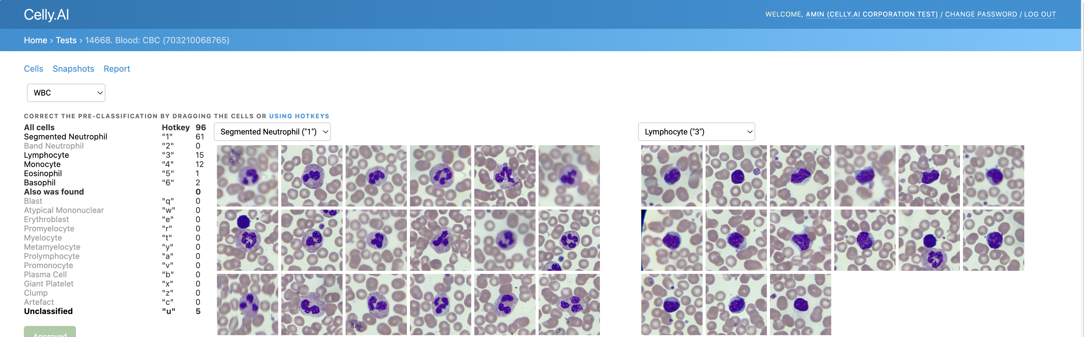
The screenshot below shows a different analysis, not malaria — but what’s important here is how many detections are triggered per frame.

In general, on iOS, it’s possible to monitor the system’s thermal state via ProcessInfo.processInfo.thermalState. In our production environment, we’ve never reached the Critical level, but the Serious level occurs regularly under very high load. For performance measurements, we used Xcode Profiler, which allows you to measure CPU, GPU, and memory load, as well as the Thermal State:

And here’s a table of thermalState values with explanations from the documentation:

| Thermal State | Recommendations | System Actions | |----|----|----| | Nominal | No corrective action required. | — | | Fair | Temperature is slightly elevated. Applications may proactively begin power-saving measures. | Photo analysis is paused. | | Serious | System performance is reduced. Applications should decrease usage of the CPU, GPU, and I/O operations. | ARKit and FaceTime lower the frame rate (FPS). iCloud backup restoration is paused. | | Critical | Applications should reduce CPU, GPU, and I/O usage and stop using peripheral devices (e.g., the camera). | ARKit and FaceTime significantly lower the frame rate (FPS). |

A full thermal and power analysis deserves a separate article — as I mentioned at the beginning, I don’t want to go too deep here. Based on publicly available sources, it can roughly be assumed that the Serious state corresponds to 80–90°C at the chip level and around ~40°C at the surface.

The iPhone works with any Bluetooth Low Energy devices. For other devices, there’s a separate flow, where the device must have an MFi (Made for iPhone) certification, operate via the iAP2 (Apple Accessory Protocol), etc. In short — that’s not our case.

It’s useful here to recall the basic roles and structure of the protocol:

• Peripheral — a device that is connected to. Usually, the peripheral sends out data or waits for a connection (examples: a watch, thermometer, heart rate monitor).
• Central — a device that connects to the peripheral. It initiates the connection, sends commands, and receives data.
• GATT (Generic Attribute Profile) — the structure through which BLE devices exchange data. GATT defines which “fields” are available, what can be read, written, or subscribed to for notifications.
• Services and Characteristics — data within a BLE connection is structured into services (logical groups) and characteristics (specific parameters). For example, a fitness tracker might have a Heart Rate service, which includes a Heart Rate Measurement characteristic (current heart rate).

In our case, the iPhone controls the stage via its built-in BLE module, which is recognized as a Peripheral with a custom GATT service and performs two tasks:

• sending movement commands to the controller for the XY axes and focus control along the Z axis
• receiving data from the controller (status, position)

Speaking of thermal load, the BLE connection should not contribute noticeably. According to data from Silicon Labs in their document on BLE power consumption, transmitting commands or receiving status at a frequency of 20 Hz (an interval of 50 ms):

• results in an increase of less than 1 mW. The iPhone XR’s typical idle power consumption is around 50–100 mW. An addition of less than 1 mW is almost negligible, especially compared to neural network processing, GPU usage, and the display.
• the radio channel is active for only about 2% of the time, sleeping the rest of the time.

We’ll dive deeper into the details of the app’s work with the BLE module and controller in the section “Working with the Motorized Stage.”

Now, a few words about the camera. We use the primary (wide-angle rear) camera: we capture H.264 video at a resolution of 1280×720 and a bitrate of about 40 Mbps.

• The higher the bitrate, the more data per unit of time → the higher the image quality. 40 Mbps is quite high for a resolution of 1280×720 (HD). It’s more than sufficient for cell analysis imaging.
• H.264 is an international video encoding standard, also known as AVC — Advanced Video Coding or MPEG-4 Part 10. It eliminates redundant data (both inter-frame and intra-frame compression), reducing the bitrate and, consequently, the file size. (Incidentally, we also had the task of recording video of the entire analysis for debugging and validation purposes.)

Thus, what we end up with is not merely a mobile UI client but a fully-fledged edge device — meaning a device that processes data locally, without constant connection to a server.

Mobile Application

Now that we’ve covered the hardware part, let’s look at how all this works at the application level. Let’s start by defining the task:

• At the input, the application receives a stream of frames from the camera — the microscope’s field of view moving across the smear.

• At the output, the application must:

• detect leukocytes (and other cells depending on the analysis)

• display detected objects with bounding boxes (BBoxes)

• perform cell counting

• send data in the background to the backend (images of cells, the scan, individual frames)

  

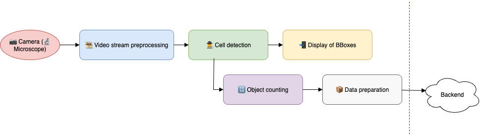
As shown in the diagram above, everything revolves around the camera frame — detection, navigation across the slide, and determining which artifacts need to be sent to the cloud all depend on it. Therefore, at the core of everything is frame stream processing. Let’s outline its main stages and key points.

1) Preprocess the frames. This includes distortion correction, artifact removal, blur level assessment, and light and color correction.

For example, each laboratory or microscope has specific lighting conditions, which can cause the neural network to malfunction. Here, it’s necessary to perform white balance normalization — by directing the field of view to an empty area and initiating the camera’s white balance adjustment.

We also had a bug where the cells were sent to the portal without color calibration. This happened because detection was launched in parallel before the camera settings were applied.

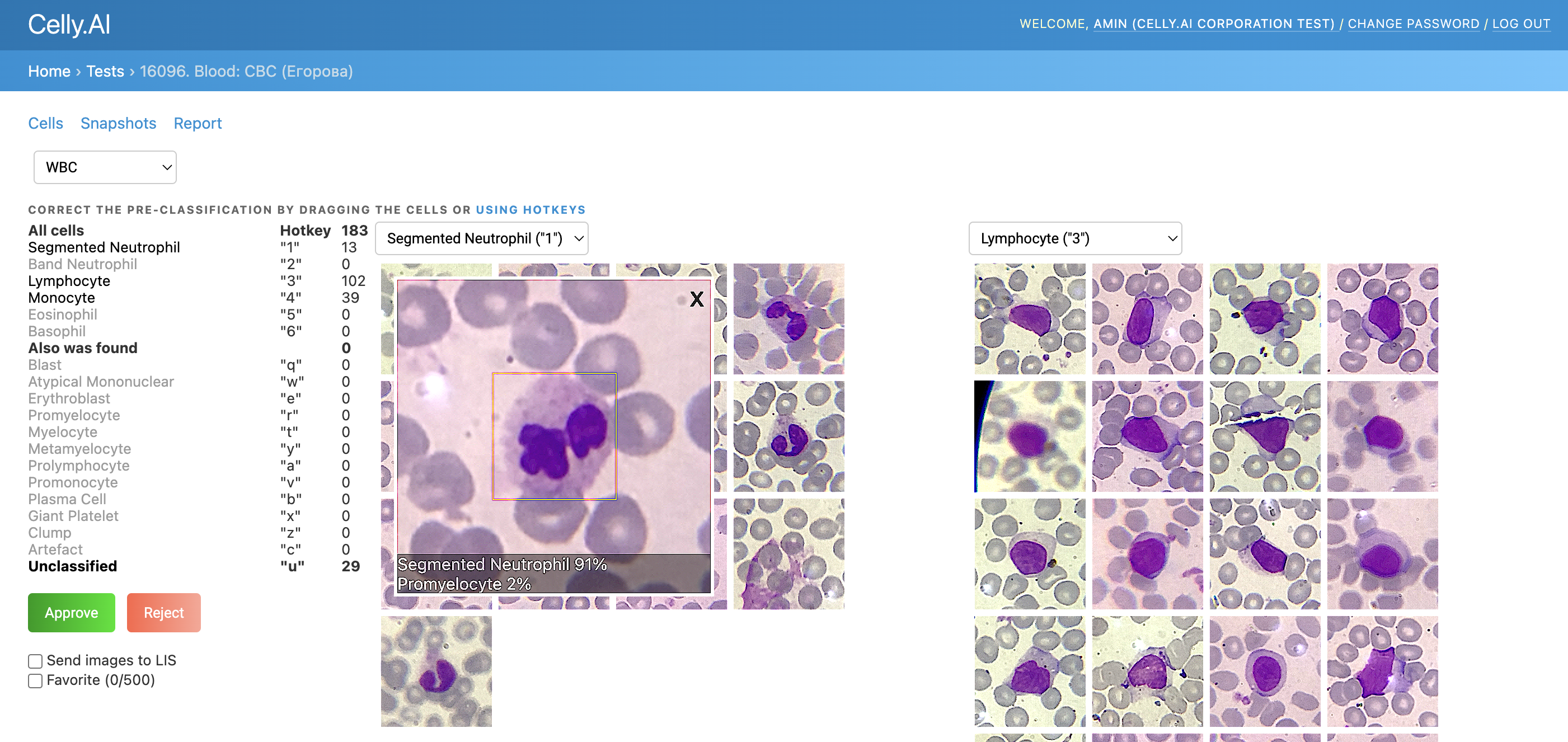
2) Detect, classify, and count cells without duplicates

For example, in the photo below, some duplicates are marked in red in one of the older analyses:

3) Control the microscope so that it moves correctly across the slide, transitions from one slide to another, and, most importantly, focuses precisely on the slide, detecting when it goes beyond the slide boundaries or lands on empty areas.

4) Upload batches of cells to the cloud (snapshots, metadata) without blocking the processing of the next analysis.

5) Repeat this process n times, as analyses are performed in batches.

6) And accomplish all of this without the phone overheating.

The application evolved in the typical startup fashion: a proof-of-concept was quickly thrown together, then refined into an MVP (Minimum Viable Product) suitable for piloting in labs and pitching to investors. As a result, the app’s architecture ended up being hybrid: some screens are implemented using UIKit-based MVP (Model-View-Presenter) screens, while new features and interfaces are written in Swift with MVVM (Model-View-ViewModel).

We use a service layer to isolate business logic: CameraService, BluetoothController, AnalysisService. All dependencies are injected either through constructors or via DI containers. In terms of reactivity and asynchronous chains with event subscriptions, we had an “evolutionary path”: we initially adopted RxSwift, then began transitioning to Combine, and with the advent of async/await, part of the chains shifted there. The result was a sort of “Frankenstein,” but we later isolated these components into separate modules so that in the future, we could simply swap out a component for a new tech stack. The entire application is interlaced with detailed logging, and for complex cases (especially those related to frame processing), we use NSLogger: it allows logging not only text but also images — which has saved us more than once when debugging the cell-processing pipeline before sending data to the server.

An entire article could be written about testing: from mocking individual parts of the analysis and quickly setting the desired states via ProcessInfo (by the way, I have a small technical note on this topic), to simulating individual steps of the analysis and covering all of it with integration and unit tests.

But let’s return to frame processing and take a look at a slightly more detailed architectural diagram than the one above:

• Analysis Controller — the decision-making center: receives frames and launches processing in the Frame Pipeline.
• Camera Service — receives the raw frame stream from the camera, transforms it, and passes it onward.
• Microscope Controller — controls the microscope’s controller.
• Frame Pipeline — a chain consisting of several stages:
• Preprocessing — correction, filtering
• Detection — object/cell detection
• Counting — counting unique objects
• Postprocessing — final filtering and preparation for visualization
• UI — responsible for displaying results to the user in real time (bounding boxes, statistics, alerts).
• Uploader — synchronizes analysis artifacts (snapshots, cells, config) with the backend.

Regarding the dependency manager: we initially used CocoaPods (which entered maintenance mode and stopped active development as of 2024), but later introduced SPM (Swift Package Manager). Some services (Computer Vision, Bluetooth, utilities) were moved into SPM modules. There were also attempts to separate ObjC/C++ code into individual xcframeworks, but there wasn’t enough time to sort it all out, so we left that code in the main project. ObjC was needed as a wrapper around C++ so that it could be called from Swift. This resulted in ObjC++ classes: their interfaces are purely ObjC, allowing Swift to interact with them, while their implementations mix ObjC and C++ code. This was before Swift supported direct calls to C++.

I should mention that I’m far from being a guru in C++ and Computer Vision algorithms, but my responsibilities included gaining a basic understanding and porting algorithms and heuristics from Python, which was where most of our R&D was conducted. I’ll describe some of those below.

Tasks

Distortion Removal

One of the adapters exhibited an optical distortion artifact in the image. As a result, a cell that should appear round would look elongated or warped, especially toward the edges of the frame. We used calibration with a chessboard grid and OpenCV’s cv::undistort() to restore the frame’s geometry:

1. We calibrate the camera — capturing images of a chessboard/grid with known geometry.

2. OpenCV computes:

3. the camera matrix K (projection parameters)

4. distortion coefficients D = [k1, k2, p1, p2, k3, …]

5. We apply cv::undistort() or cv::initUndistortRectifyMap() + remap():

6. this computes where each point “should have landed” in reality

7. the image is “straightened” back to correct geometry

   

Later on, the adapter was replaced — this step was removed.

Determining Position on the Slide

To accurately count cells, it’s crucial to know their coordinates as precisely as possible. In the video here, you can see what happens when the shift determination is incorrect.

Initially, we tried calculating the relative shift between two frames and summing up the absolute shift. We tested several approaches:

• the classic image registration method via phase correlation based on the Fast Fourier Transform. We implemented this in OpenCV and even used Apple Accelerate.
• methods based on local keypoints with descriptors: SURF, SIFT, ORB, and others.
• Optical Flow
• Apple Vision’s built-in VNTranslationalImageRegistrationRequest

On one hand, we had some assumptions:

• no scaling or rotations were present
• optically: a clean, unblurred smear, without empty areas

Despite this, there were still issues due to changes in lighting, focus, accumulated error, abrupt shifts, noise, or artifacts in the image.

This resulted in a comparison table like the one below:

Here’s your precise translation of the provided table and text:

| Method | Advantages | Disadvantages | Usage Notes | Speed | Comment | |----|----|----|----|----|----| | FFT + cross-correlation (OpenCV, Accelerate) | Very fast, global shift detection, simple to implement | Accumulates error, not robust to abrupt shifts | Requires images of identical size, suitable for “pure” shifts | Very high | Used as the primary method | | SIFT | High accuracy, scale/rotation invariant | Slow, used to be non-free | Excellent for diverse scenes with texture and complex transformations | Slow | Experimental option | | SURF | Faster than SIFT, also scale/rotation invariant | Proprietary, not always available | Slightly better suited for real-time but still “heavy” | Medium | Experimental option, especially since under patent | | ORB | Fast, free, rotation invariant | Sensitive to lighting, not robust to scale changes | Works fairly well for image stitching | High | Before we moved stitching to the cloud, we had versions using this | | Optical Flow (Lucas-Kanade) | Tracks movement of points between frames, good for video | Doesn’t handle global transformations, sensitive to lighting | Best in videos or sequences with minimal movement | Medium | We experimented with this for digitization (stitching) of images | | Optical Flow (Farneback) | Dense motion map, applicable to the whole image | Slow, sensitive to noise | Good for analyzing local motions within a frame | Slow | We experimented with this for digitization (stitching) of images | | Apple Vision (VNTranslationalImageRegistrationRequest) | Very convenient API, fast, hardware-optimized | In our case, accuracy was poor | Perfect for simple use cases on iOS/macOS | Very high | We tried it and abandoned it |

For each option, we tried to find the optimal configuration in terms of accuracy and performance for comparing against a reference shift: we varied image resolutions, algorithm parameters, and different camera and microscope optics settings. Below are a couple of charts from these kinds of experiments.

And here’s what the debugging process looked like for detecting keypoints, which we later intended to use for calculating the shift.

As a result, once the robotic stage was introduced into our system, we began using the coordinates from its controller, which we then refined using CV heuristics.

Cell Counting

Essentially, the task of cell counting is a specific case of object tracking & deduplication: “to identify what the cell is, avoid counting it twice, avoid overcounting, and not miss the necessary cells — all in fractions of a second, in real time via the camera and running on the phone’s hardware.” Here’s how we solved it:

1. Object Detection. We use neural networks to detect objects in the frame (Bounding Box, BB). Each BB has its own confidence score (network confidence) and cell class.

   

To combat background noise and false positives, we apply fast filtering:

• color-based: for example, by intensity or color range. For instance, here on the left, a red highlight marks an erythrocyte — but the neural network initially classified it as a leukocyte.

• However, color filters came into play afterward, and it was filtered out.

  

A red highlight marks an erythrocyte discarded by the filters.

• geometric: we discard objects whose sizes fall outside typical cell dimensions.

• we also discard cells that partially extend beyond the frame edges — those are of no interest to us

  

1. Counting unique objects. Some BBs may be counted more than once for the same cell, so it’s important to detect such cases and count them only once. At one point, we were inspired by a guide from MTurk that describes two options:

   Option 1: Compare the distances between BB centers — if a new BB is too close to one already recorded, it’s likely “the same” cell.

   Option 2: Calculate IoU (intersection over union, Jaccard Index) — the metric for overlap between rectangles. If a new BB overlaps significantly with an existing one, we count it only once.

   

In general, it’s necessary to maintain object tracking between frames, especially if we revisit previously scanned areas of the smear. Here again, it’s critically important to accurately determine the position on the slide — otherwise, the entire count goes down the drain.

Digitization

One of the tasks was digitizing the scan, essentially creating a software-based histology scanner for the smear. The photo below shows what it looks like: arrows indicate the movement used to build the scan, where we capture frames and stitch them into one large image.

Movement of the field of view across the smear

Here again, accurate position determination was critically important, followed by seamless stitching.

It’s worth noting that initially we didn’t have a motorized stage and relied on manual navigation. Imagine trying to assemble a mosaic from hundreds of fragments. If you miss the coordinates, the mosaic ends up misaligned.

Here’s what the first experiments looked like: jumping fields of view, seams, differences in lighting, empty spaces.

On the left — a map with uneven brightness and exposure, where “seams” are visible at the frame junctions. On the right — unevenly stitched tissue images with gaps.

Or, for example, a user scans the smear, moving quickly across it — some areas end up blurred (Motion Blur). We tried discarding such frames if they didn’t meet the acceptable blur threshold or if the shift couldn’t be calculated for them.

Blurred frames overlaid on the scan during abrupt movement

Gradually, we progressed toward the following approach:

There were many iterations: stitching on the device, using different methods, at various frame resolutions and camera configurations. We eventually arrived at the solution where the scan is assembled in the cloud, and the mobile device sends frames with calibrated white balance and exposure.

Below is an example of how we measured the processing speed of individual frame-processing components depending on the configuration: camera settings, selected algorithms, and their parameters. (there’s some mixing with Russian here, but I hope the overall idea is clear)

Working with the motorized stage

Now — the details about the connection between the iPhone and the motorized stage: how we communicate over BLE, what commands we send, and how we configured autofocus. The mobile device connects via Bluetooth to the controller on the stage and moves along the XYZ coordinates. More precisely, it’s the stage itself that moves, but from the perspective of the image seen through the objective lens by the mobile device, it looks like the movement happens across the slide.

Our stage is also custom-built — not because we “want to make everything ourselves,” but because commercial solutions start at $10,000, and that’s no joke. We hired a design bureau and built our own version for about ~$800. It turned out significantly cheaper because one of the engineers noticed in time that the construction of a motorized microscope stage suspiciously resembles a 3D printer. Same XYZ kinematics, same stepper motors, same rails. As a result, we’re using mass-produced and inexpensive components, but tailored to our specific requirements. Structurally, the stage consists of three parts: the XY platform itself, the focusing block (Z-axis, where the motor is attached to the fine focus knob), and the control unit — the controller that receives commands via Bluetooth and sends them to the stepper motors. All of this works in conjunction with the mobile device.

Components of the motorized microscope stage

For manual stage movement, we use a virtual joystick (displaying movement buttons to the user on the screen) — it’s used in calibration and system setup scenarios. However, during analysis, control is always automated. Here’s how the joystick worked in the first versions — later, we enhanced it with sound and delay handling.

Communication Protocol

As the Bluetooth interface, we use the HC-08 board. The BLE module operates by default in text terminal mode, meaning requests and responses simply pass back and forth. For configuration and system tasks (changing the name, communication speed), AT commands are used.

The controller itself runs firmware based on GRBL, using G-code commands. The main scenarios here are:

• initializing the connection (the phone must detect that the stage is connected)

• scanning the slide (moving the stage along all axes)

• stopping/resuming scanning

• handling exceptional situations: reaching the limit switch, interrupting movement, command buffer overflow. There’s a separate document covering error handling.

  

GRBL has its own set of commands that start with the $ symbol, for example:

• $H — homing or calibration and seeking the hardware zero via limit switches. Usually performed at initial startup and later as needed if significant accumulated error occurs during movement.
• $J=<command> — Jogging mode, which simulates joystick control. The command itself should describe relative movement along all axes. An example of such a command: $J=G21G91Y1F10
• G21 — units in millimeters
• G91 — relative positioning
• Y1 — movement along the Y-axis by 1 millimeter
• F10 — movement speed.
• ? — GRBL status query. Returns a string with the machine’s key parameters. Example response: <Alarm|MPos:0.000,0.000,0.000|FS:0,0|Pn:XYZ|WCO:-5.300,0.000,-2.062>

We’re interested in the first two parameters:

• status. It can be “Idle,” “Running,” or “Alarm.”
• MPos — the current position of the stage.

I won’t go too deep into GRBL and the stage control protocols — that’s material for a separate article. In short: GRBL is an open-source firmware from the CNC world, perfectly suited for controlling three-axis systems (XY+Z) via simple G-code commands. We chose the simplest possible BLE module — the HC-08 — to avoid dealing with MFi and iAP. It was crucial for us that the iPhone could reliably send commands and receive status updates with minimal latency, without significantly increasing the cost of the kit.

Tasks

Autofocus

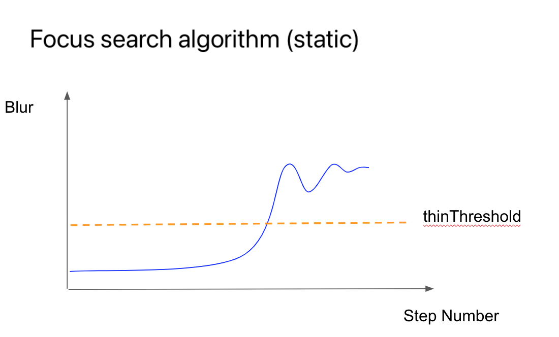
Earlier, I mentioned focusing. This process is performed periodically during smear scanning because the specimen is applied unevenly, which is especially noticeable at high magnifications. It’s necessary to monitor the level of blur and adjust the focus in time. Here’s how it works.

The graph below shows the relationship between focus level and time. We start with a blurred image, gradually moving the stage to the optimal focus position.

Scanning

I already mentioned digitizing the scan on the mobile side. It’s worth noting here that digitization can be performed at different magnifications: from 5x to 40x. At lower zoom levels, it’s easier to navigate and detect the boundaries of the smear, while at higher magnifications, the cellular details become visible.

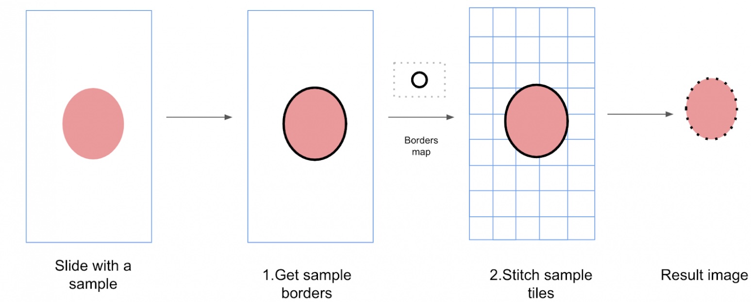
In our case, we work with two levels:

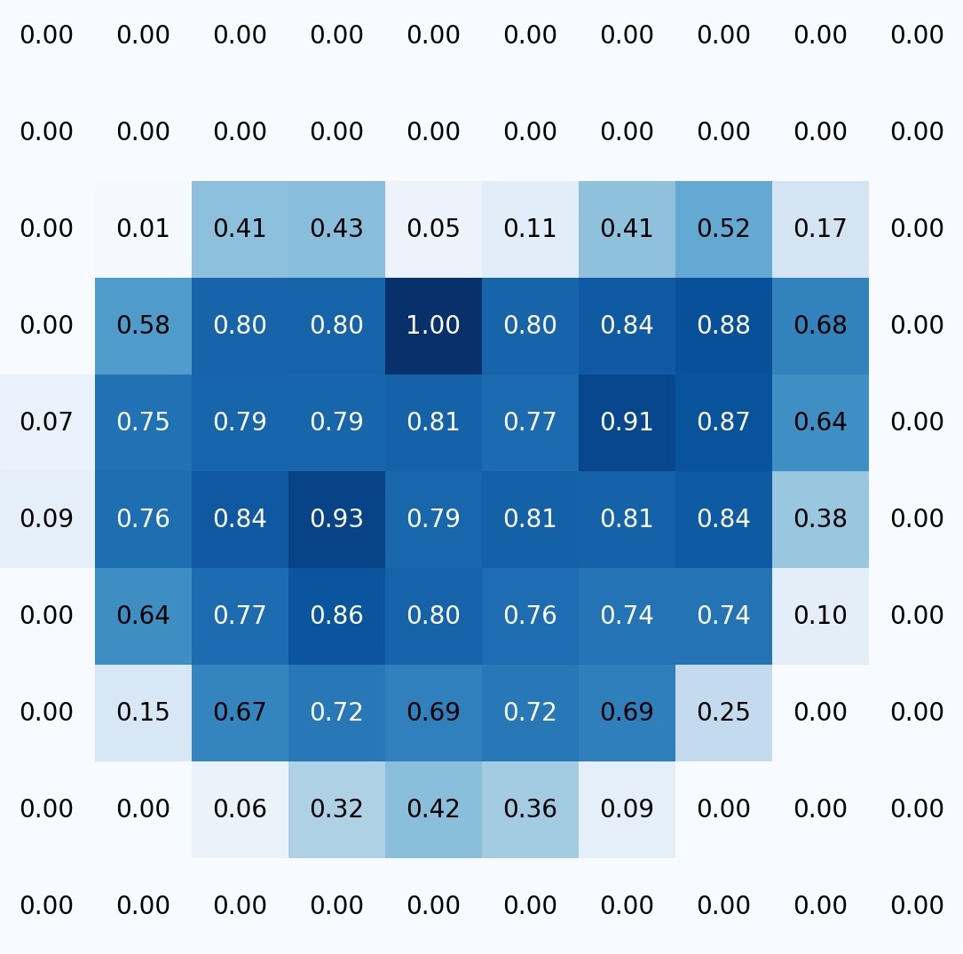
1. Boundary detection at 4x magnification. The algorithm scans the entire slide, determines the smear area, and generates a boundary map for the next stage. The output is something like a heat map. For example, from the low-magnification image on the left, we obtain a matrix that we then use to plan the steps for navigating at higher magnification:

   

   

2. Scanning the smear at 20x magnification (or another level). The algorithm scans and saves images for subsequent assembly into a single map. Scanning proceeds line by line, within the boundaries of the smear. A photo is captured for stitching when:

3. the image is in focus

4. the controller is in an idle state, i.e., not moving

   

So that the user doesn’t have to switch objectives each time, we perform boundary detection and scanning across all slides in the batch simultaneously, while uploading the previous batch to the cloud in parallel. The stitching or assembly of the image then takes place in the cloud, but that’s a topic for a separate article.

Conclusion

This project demonstrated that even a smartphone from 2018 can handle tasks that previously required desktops, servers, and expensive automated microscopes. Of course, there’s still a lot left behind the scenes: from dataset collection to fine-tuning exposure settings. If you’re interested, I’d be happy to cover that separately. Feel free to ask questions, share your own experiences, and perhaps together we’ll create a follow-up or dive deeper into specific aspects. Thanks for reading!

👋 Let’s Connect!

Ansar

• Email: ansaril3g@gmail.com
• LinkedIn: Ansar Zhalyal
• Telegram: @celly_ai

Amin

• Email: amin.benarieb@gmail.com
• LinkedIn: Amin Benarieb
• Telegram: @aminbenarieb

\

This content originally appeared on HackerNoon and was authored by Amin Benarieb

Print Share Comment Cite Upload Translate Updates

APA

Amin Benarieb | Sciencx (2025-07-09T06:01:02+00:00) How We Turned the iPhone into a Laboratory Microscope with AI and BLE. Retrieved from https://www.scien.cx/2025/07/09/how-we-turned-the-iphone-into-a-laboratory-microscope-with-ai-and-ble/

MLA

" » How We Turned the iPhone into a Laboratory Microscope with AI and BLE." Amin Benarieb | Sciencx - Wednesday July 9, 2025, https://www.scien.cx/2025/07/09/how-we-turned-the-iphone-into-a-laboratory-microscope-with-ai-and-ble/

HARVARD

Amin Benarieb | Sciencx Wednesday July 9, 2025 » How We Turned the iPhone into a Laboratory Microscope with AI and BLE., viewed ,<https://www.scien.cx/2025/07/09/how-we-turned-the-iphone-into-a-laboratory-microscope-with-ai-and-ble/>

VANCOUVER

Amin Benarieb | Sciencx - » How We Turned the iPhone into a Laboratory Microscope with AI and BLE. [Internet]. [Accessed ]. Available from: https://www.scien.cx/2025/07/09/how-we-turned-the-iphone-into-a-laboratory-microscope-with-ai-and-ble/

CHICAGO

" » How We Turned the iPhone into a Laboratory Microscope with AI and BLE." Amin Benarieb | Sciencx - Accessed . https://www.scien.cx/2025/07/09/how-we-turned-the-iphone-into-a-laboratory-microscope-with-ai-and-ble/

IEEE

" » How We Turned the iPhone into a Laboratory Microscope with AI and BLE." Amin Benarieb | Sciencx [Online]. Available: https://www.scien.cx/2025/07/09/how-we-turned-the-iphone-into-a-laboratory-microscope-with-ai-and-ble/. [Accessed: ]

rf:citation

» How We Turned the iPhone into a Laboratory Microscope with AI and BLE | Amin Benarieb | Sciencx | https://www.scien.cx/2025/07/09/how-we-turned-the-iphone-into-a-laboratory-microscope-with-ai-and-ble/ |

Please log in to upload a file.

There are no updates yet.
Click the Upload button above to add an update.

You must be logged in to translate posts. Please log in or register.