
This content originally appeared on Level Up Coding - Medium and was authored by Guilherme Ziegler
Introduction
In recent years, betting has transformed into a global digital industry, raising significant public health concerns. The widespread availability of online platforms and mobile access has made gambling more accessible than ever, effectively creating what experts describe as a “casino in your pocket” (WHO, 2024).
Among the various forms of gambling, slot machines, particularly digital ones, are considered especially risky. Their rapid gameplay, continuous reinforcement, and instant rewards are strongly linked to addictive behaviors, which makes them one of the main drivers of problem gambling worldwide (Techopedia, 2024).
The scale of the issue are significant. Global estimates suggest that around 1.2% of adults suffer from gambling disorder, while many others experience financial, psychological, and social harm due to gambling-related activities (WHO, 2024).
At its core, the question is whether betting can generate consistent long-term returns. The most rigorous way to answer this is through mathematics.
Casino games are designed around a inherent statistical advantage known as the house edge, which ensures that, over time, expected returns are negative for the player.
While short-term wins are possible and often emphasized, probability theory makes it clear that repeated play leads to predictable losses rather than sustainable gains.
For those familiar with my previous articles, I am an economist and data scientist working in financial risk, and I enjoy raising thought-provoking questions for discussion.
In this article, we explore the key mathematical principles that demonstrate why consistent long-term profits from betting are unlikely. To make this concrete, we also build a simple online casino using Python and Streamlit.
We do this by:
- Explaining the math and statistics behind long-term returns in digital slot machines.
- Coding a basic casino model in Python and running the game in Streamlit, which is engaging to play.
- Running simulations for multiple players on a single slot machine.
Article Structure
This article has three sections:
- Maths and equations.
- Python functions to run the game.
- Streamlit integration.
The first section presents mathematical theory behind online betting, especially in casino systems.
The second demonstrates how to build a simple slot machine for experimental purposes, covering the core backend logic that powers the game.
The third focuses on a basic frontend implementation to render the application for single-player and multiplayer modes, where I demonstrate some insights about betting in the short and long term.
In this section, we’ll explore the key concepts behind betting in a slot machine game:
- Symbols and weights.
- Winning positions.
- Expected payout.
- RTP (Return to Player).
Symbols and weigths
In a slot game, symbols represent the outcome of a single spin. Each time the slot is played, every symbol has a probability of appearing on the screen.
This probability is determined by a set of predefined weights, in other words, how rare each symbol is relative to the others.
To make this clear, consider a machine with seven different symbols, ordered by rarity: tiger, gold, clover, star, seven, wild, and jackpot.
Also, let’s assume default weights are given as follows:
SYMBOLS = ["tiger", "gold", "clover", "star", "seven", "wild", "jackpot"]

SYMBOL_EMOJI = {"tiger":"🐅","gold":"💰","clover": "🍀",
                "star":"⭐","seven":"7️⃣","wild":"🎰",
                "jackpot":"💎"}

DEFAULT_WEIGHTS = [5, 5, 5, 5, 1, 0.3, 0.5]
The initial weight configuration is heavily skewed toward low-tier symbols, with tiger, gold, clover, and star all assigned equal and dominant weights (5), meaning they will appear very frequently and define most of the player experience.
In contrast, higher-value symbols like seven (1), jackpot (0.5), and especially wild (0.3) are significantly rarer, which is a typical design choice to preserve excitement and control payouts.
Think of weights as “tickets in a draw.” The more tickets a symbol has, the more often it shows up.
Instead of working with probabilities for each symbol we normalize the weights to get them, equation 1:
- pi is the probability of symbol i appearing;
- wi is the initial weight assigned to symbol i (controls how frequent it is);
- N is the number of initial symbols (5 in this case) ;
- J is the index used to iterate over all symbols;
- And the term in the summation represents the total weight across all symbols, acting as the normalization factor.
Intuitively, you take the weight of one symbol and divide it by the total weight of all symbols to get its probability.
We could start directly with probabilities, some would need to be extremely small, making them difficult to discuss.
Let’s take the tiger and jackpot as examples (see Equation 2):
the probability of getting one tiger is 18.66% while the probability of one jackspot is 1.87%, way rarer.
Winning positions
As the saying goes:
One swallow does not make a summer.
Neither a tiger alone.
This brings up the concept of winning positions.
A winning position is a rule that establishes how many matching symbols must appear together, and in which positions, for a prize to be paid.
Usually, this number is three for common slot machines, but it can be set to any value. In a game based on a 1 × 3 matrix, the columns indicate the positions where a symbol can appear. A win occurs when three matching symbols are displayed on the screen simultaneously.
Since all 3 symbols have the same probability of appearing once, we come up with equation 3:
For this particular case a jackspot winning position happens approximately once 1 in 153,846 chances.
Why is the probability of a wild lower than that of a jackpot?
In this game, the wild symbol acts as a substitute, meaning it can complete a winning position when combined with a matching pair of another symbol. Because of this flexibility, it contributes to many more winning combinations than a regular symbol.
To keep the game balanced, the wild must appear less frequently than the jackpot. Even though it shows up less often, when it does appear, it significantly increases the chances of forming a winning position.
Since we have defined a winning position in this 1 x 3 matrix game, adding more lines increases the overall chance of winning. Each line is independent, meaning the outcome of one line does not affect another.
However, these events are not mutually exclusive, since multiple lines can win at the same time. Because of that, we cannot simply sum their probabilities.
Instead, the correct approach is to compute the probability of winning in at least one line using the complement rule, by calculating the probability that all three lines lose simultaneously and subtracting it from one.
Therefore, the probability of getting at least one winning line with a 3 x 3 matrix game is given by equation 4:
Where i represents any symbol, and L is the number of winning lines — here, 3 horizontal lines. The exponent 3 comes from Equation (3), since a winning line requires three identical symbols. The term inside the brackets is the probability of losing on a single line.
Now that we understand the classic example, let’s add some more fun to the game. Considering only the chance to win horizontally is not ideal in terms of user experience and gameplay. We need to add more fun so that the slot machine becomes more attractive to players.
One way to do so is to define a couple of additional winning positions. For now, we are focused on horizontal lines, but we could also consider moving vertically, in terms of columns, as well as diagonals, and maybe some left and right triangles to keep the mood high.
Here is a representation of all possible winning lines in a 3 × 3 game, , Figure 2.
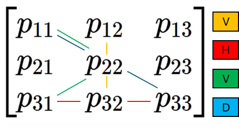
We see that there are 4 possible winning positions, represented by rectangles: V (vertical), H (horizontal), D (diagonals), and > (left triangle).
Each V can occur 3 times, since there are 3 columns; the same goes for H, with 3 horizontal lines. In a matrix, there are only 2 possible diagonals, and the triangle can occur on the left side, as depicted above, but also on the right side.
Thus, summing 3V + 3H + 2D + 2> gives 10 winning positions in a single spin.
Wherever the odds are for each symbol to appear, there are 10 possible configurations that will pay the prize.
From that we define another hiperparameter and can update the initizaliation of the game:
SYMBOLS = ["tiger", "gold", "clover", "star", "seven", "wild", "jackpot"]
pyth
SYMBOL_EMOJI = {"tiger":"🐅","gold":"💰","clover": "🍀",
                "star":"⭐","seven":"7️⃣","wild":"🎰",
                "jackpot":"💎"}

DEFAULT_WEIGHTS = [5, 5, 5, 5, 1, 0.3, 0.5]

WINNING_POSITIONS = 10
Expected payout
Previously, we defined how to win in the game, but how much a win pays is yet to be set.
Since each symbol has a certain rarity of being displayed on the screen, it is intuitive to assume that the rarer the symbol, the higher the payout.
So, taking tiger, gold, clover, star, and seven as examples, we could assume that the star pays more than all of them. However, since tiger, gold, and clover are equally frequent in the game, they should pay the same, right?
That makes sense, but once again, our game would become boring. Therefore, we must configure a hyperparameter that determines the payout for each symbol in a winning position, while still encouraging the player to root for the higher-paying symbol, even when the odds are the same.
This is achieved by setting default multipliers as follows:
DEFAULT_MULTIPLIERS = {"tiger": 12,
                       "gold": 14,
                       "clover": 16,
                       "star": 18,
                       "seven": 25,
                       "wild": 0,
                       "jackpot": 0}
Note now that star is as weel as frequent as tiger but pays aditional 6 units in return. Seven , is 5 times rarer than the precedent ones, and pays aditional 13 units when compared with tiger.
Why do wild and jackpot pay nothing back?
As mentioned above, the wild works as a substitute, so on its own it pays nothing. We must ensure that whenever a winning position can be formed using a wild, the highest possible prize is paid.
That said, in a case where both a tiger winning position and a seven winning position could be formed using a single wild, we assume it will form the higher-paying combination, and in this case, bind it to that outcome.
The jackpot has a similar behavior: it pays nothing directly because, when it appears in a winning position, the player receives the accumulated prize, which is funded by a fraction of each bet.
In this case, the rarer the odds of a winning position, the higher the total prize paid out.
We covered that each symbols pays back differently, but they always should pay back more than the overhall bet for a winning position.
We define 10 as the number of winning positions, so when we bet, let’s say, $10 per spin, we are dividing the value of bet for the number of 10 possible winning positions.
It means that for each $10 bet, we are allocating $1 to a winning position that, when displayed on the screen, is multiplied by the default multiplier.
Thus, if we win with tiger, we get $12 back; if we win with clover, we get $16 back; and of course, if we win with both, the total payout is $28 from a $10 bet.
In terms of the risk–reward ratio, we have 1:2.6, for each dollar we bet, we expect to receive $2.6 back.
Note that default multipliers are hyperparameters, and each should be set such that the multiplier times 10% of the total bet exceeds the original bet. This is a default constraint for the total number of winning positions we have.
To make this clear, tiger pays $12 for each $1 when the total bet is $10. Therefore, when a single tiger wins, the minimum payout is $12 × $1, which must be greater than — and indeed is greater than — $10.
Since we intuitivelly undertood the dynamics of the payouts, let’s formalize the expected payout for any winning lines in equation 5:
Where:
- E[payout] is the expected total payout;
- B is the total bet per spin (e.g., $10);
- W is the total number of possible winning positions (e.g., 10);
- k is the number of winning positions observed in the experiment (e.g., 1);
- mi is the multiplier paid when symbol i forms a winning position.
Now, as an example, for one winning position formed by three tigers, with a total bet of $10 and 10 possible winning positions, we obtain an expected payout of $12 (see Equation 6).
RTP (Return to Player)
We have covered symbols and their weights, winning positions, and expected payouts — all the elements needed to estimate the Return to Player (RTP) in the long run.
For any given spin, there are only two possible outcomes: either the player loses the entire bet or wins an amount greater than the original stake.
Since each symbol has an associated probability (pi) and we have defined all possible winning positions (wp), RTP represents the average amount of money returned to the player over many spins.
To compute the Return to Player (RTP), we take the expected payout over all possible winning outcomes.
In this setup, each winning position receives 10% of the total bet, and a win requires three identical symbols. Therefore, the probability of a winning combination for symbol i is pi³ (see equation 1).
Each symbol also has an associated multiplier mi, which defines its payout. By combining these elements, the RTP simplifies to:
This means the RTP is simply the sum, over all symbols, of the probability of hitting three of that symbol multiplied by its respective payout multiplier.
In other words, RTP represents the average return per unit bet in the long run.
There are three possible outcomes for the RTP in a slot machine game:
- If it is greater than 1, the player wins more than they bet.
- If it is equal to 1, the player breaks even over time — a scenario that offers little incentive to play.
- If it is less than 1, the player loses more money than they win in the long run.
Yes, it does. Since the RTP is set slightly below 1, the game is designed to make players feel like they are winning — because each individual win pays more than the original bet. However, wins are rare enough that the total return remains below 1 over time.
Remember those hyperparameters from earlier? They are carefully calibrated to create the feeling of “I might win today.” In the short run, it is entirely possible to achieve high returns due to randomness, driven by the symbol weights. However, over time, the player typically gives back all winnings and eventually loses the initial stake.
Furthermore, some games can be configured to have an RTP greater than 1 for a limited number of spins, and then revert to below 1 in order to recover the house’s expected profit.
In practice, let us assume 5 spins, each with a $10 bet, where each spin either returns a payout or 0 (see Equation 7). This empirically simulates the process.
For these 5 spins, the payouts are 12, 0, 16, 0, and 20, summing to $48 returned out of $50 wagered. The resulting RTP in this case is 0.96, which is quite close to what slot machines are typically calibrated to achieve.
For 5 spins, the payouts are 12, 0, 16, 0, and 20, summing to $48 returned out of $50 wagered. The resulting RTP is 0.96, which is quite close to what slot machines are typically calibrated to achieve.
The winning rate in this case is 3 out of 5, meaning the player wins 60% of the spins, yet still loses $2 over those 5 spins. In the long run, if this RTP remains constant, after more 44 spins the player would be expected to lose the entire initial amount wagered.
So, Good luck!
Coding a slot machine in python and streamlit
Based on what we’ve built so far, here’s a clear way to guide the reader through the code:
We’ve already covered the core logic behind a slot machine game. Now, it’s time to translate those concepts into a working web application using Python.
Some parts of the code reuse ideas explained in earlier sections, so they’ll be referenced briefly to avoid unnecessary repetition.
This section is organized into the following topics:
- Required libraries.
- Initial setup and parameters.
- Game functions.
- Streamlit interface.
Required libraries
Below is the complete list of libraries used in this project, organized by their role in the application:
import streamlit as st

import pandas as pd
import numpy as np

import plotly.express as px
import matplotlib.pyplot as plt
from matplotlib.animation import FuncAnimation, PillowWriter
import plotly.graph_objects as go

from scipy.optimize import minimize

import random
import time
import hashlib

from typing import List, Tuple
from collections import Counter
Streamlit powers the web interface, handling user input, layout, and real-time interaction.
Pandas and NumPy support data handling and numerical operations, making it easy to manage game state and calculations.
Plotly and Matplotlib are used for visualization, Plotly for interactive charts within the app, and Matplotlib for more controlled or animated graphics. SciPy provides optimization tools, useful for tuning parameters and simulations.
Finally, standard libraries like random (game randomness), time (timing control), and hashlib (deterministic hashing) support core game mechanics.
Initial setup and parameters
We start by defining the symbol system, which represents the core of the slot machine. Each symbol has a name, a visual emoji representation, a payout multiplier, and a probability weight that controls how often it appears.
SYMBOLS = ["tiger", "gold", "clover", "star", "seven", "wild", "jackpot"]
SYMBOL_EMOJI = {"tiger":"🐅","gold":"💰","clover":"🍀","star":"⭐","seven":"7️⃣","wild":"🎰","jackpot":"💎"}
DEFAULT_MULTIPLIERS = {"tiger": 12, "gold": 14, "clover": 16, "star": 18, "seven": 25, "wild": 0, "jackpot": 0}
DEFAULT_WEIGHTS = [5, 5, 5, 5, 1, 0.3, 0.5]

INITIAL_BALANCE = 1000
WINNING_POSITIONS = 10
- SYMBOLS: defines all possible outcomes in the slot machine, representing the full set of symbols that can appear during a roll.
- SYMBOL_EMOJI: maps each symbol to its visual representation, used to render the interface in a more intuitive and engaging way.
- DEFAULT_MULTIPLIERS: controls the payout value associated with each symbol, directly impacting reward calculation when winning combinations occur.
- DEFAULT_WEIGHTS: defines the probability distribution for each symbol, determining how frequently each outcome appears during random selection.
- INITIAL_BALANCE: sets the starting amount available to the player before any bets are placed or rounds are played.
- WINNING_POSITIONS: defines how many positions are evaluated in the game grid when checking for winning combinations.
These parameters act as the foundation of the game, ensuring consistency across each run.
The Wild and Jackpot symbols are special cases: they are reserved to modify gameplay dynamics. The Wild increases the chances of forming winning combinations, while the Jackpot is tied to the highest reward, representing the grand prize for a lucky outcome.
I previously configured the game to make it fun and balanced to play. This initial configuration can be adjusted by the game owner, depending on the desired experience or difficulty.
In the next sections, I will show a step-by-step approach to optimize these parameters for a target RTP (Return to Player). For now, we will assume they represent a fair starting point.
Game functions
Now, let’s move on to the core functions of the application. We gradually increase in complexity as we proceed.
def generate_seed() -> str:
    return str(random.random())

def hash_seed(seed: str) -> str:
    return hashlib.sha256(seed.encode()).hexdigest()
The first function generate_seed() creates a random value using random.random() and converts it into a string. It simply returns a random number as text.
The second function hash_seed() takes a seed, encodes it with seed.encode(), and then applies hashlib.sha256() to generate a fixed-length hash. The result is returned as a hexadecimal string using .hexdigest().
def spin(seed: str, weights: List[float]) -> List[str]:
    rng = random.Random(seed)
    return rng.choices(SYMBOLS, weights=weights, k=9)
The function spin() simulates a random “spin” using a controlled seed.
It creates a deterministic random generator with random.Random(seed), meaning the same seed will always produce the same results.
Then it uses rng.choices() to select 9 items from SYMBOLS, following the probability distribution defined by weights.
The result is a list of 9 randomly chosen symbols, in other words, the output of a user interecation with the slot machine.
def get_positions(grid: List[List[str]]) -> List[List[str]]:
    positions = []
    positions.extend(grid)
    for col in range(3):
        positions.append([grid[row][col] for row in range(3)])
    positions.append([grid[i][i] for i in range(3)])
    positions.append([grid[i][2-i] for i in range(3)])
    positions.append([grid[0][0], grid[1][1], grid[2][0]])
    positions.append([grid[0][2], grid[1][1], grid[2][2]])
    return positions
The function get_positions() is built to extract all possible winning patterns from a 3x3 grid in a single spin.
We can classify these patterns into four groups:
- Vertical lines (V): 3 columns → each column forms one possible line
- Horizontal lines (H): 3 rows → each row is already included directly from the grid
- Diagonals (D): 2 main diagonals
- Triangles (>): 2 additional asymmetric patterns formed by selecting corners with the center
So the function collects:
- 3 vertical positions by iterating over columns
- 3 horizontal positions directly from the grid
- 2 diagonal positions ([grid[0][0], grid[1][1], grid[2][2]] and [grid[0][2], grid[1][1], grid[2][0]])
- 2 triangular patterns (left and right skewed combinations)
In total, this results in 10 possible winning positions per spin, represented as different ways of traversing the same 3x3 matrix.
Next, we move to the function calculate_payout .
def calculate_payout(
    result: List[str],
    bet: float,
    multipliers: dict,
    size: int,
    show_winning_positions: bool = True
    ) -> float:

    grid = [result[i:i+size] for i in range(0, size * size, size)]
    positions = get_positions(grid)

    bet_per_position = bet / len(positions)
    payout = 0.0
    winning_positions = []

    def is_full_line(line, symbol):
        return all(s == symbol or s == "wild" for s in line)

    def evaluate_line(line):
        nonlocal payout

        if line.count("jackpot") == len(line):
            line_payout = st.session_state.jackpot
            payout += line_payout
            st.session_state.jackpot = 0
            winning_positions.append(f"JACKPOT line = ${line_payout:.2f}")
            return

        wild_count = line.count("wild")
        non_wild = [s for s in line if s not in ("wild", "jackpot")]

        if not non_wild:
            return

        unique_symbols = set(non_wild)
        line_len = len(line)

        if len(unique_symbols) == 1:
            symbol = non_wild[0]
            total_count = non_wild.count(symbol) + wild_count

            if total_count == line_len:
                line_payout = bet_per_position * multipliers.get(symbol, 0)
                payout += line_payout
                winning_positions.append(f"{symbol} line = {line_payout:.2f}")

        elif len(unique_symbols) == 2 and wild_count > 0:
            best_payout = 0
            best_symbol = None

            for symbol in unique_symbols:
                count = non_wild.count(symbol)
                total_count = count + wild_count

                if total_count == line_len:
                    line_payout = bet_per_position * multipliers.get(symbol, 0)
                    if line_payout > best_payout:
                        best_payout = line_payout
                        best_symbol = symbol

            if best_payout > 0:
                payout += best_payout
                winning_positions.append(f"{best_symbol} line (with wild) = {best_payout:.2f}")

    for line in positions:
        evaluate_line(line)

    if show_winning_positions and winning_positions:
        st.write("Winning positions:")
        for wl in winning_positions:
            st.write(f"  {wl}")

    return payout
This function is responsible for calculating the total payout of a spin in a grid-based slot system. The grid is first reconstructed from a flat result list into a square matrix using the provided size, splitting the list into rows of equal length.
After that, all possible winning patterns are extracted through the function get_positions(grid), which returns rows, columns, diagonals, and any additional predefined paylines.
The total bet is then evenly distributed across all available positions, resulting in a bet_per_position value used for individual line evaluation. This is done because, within a single spin, there are 10 possible winning outcomes.
Each line is evaluated independently inside the evaluate_line function:
If the entire line is composed of "jackpot", the global jackpot stored in st.session_state.jackpot is awarded to the player and immediately reset to zero. This represents the highest possible win condition. Once a jackpot hits, no other winning positions are considered for that spin.
For regular evaluation, the function separates wild symbols from normal symbols and ignores "jackpot" in standard calculations. If a line contains only wilds or jackpot symbols, it is skipped.
When a line contains a single unique symbol (plus possible wilds), the function checks whether the combination of that symbol and wilds completes the full line. If so, the payout is calculated using the corresponding multiplier from the multipliers dictionary.
A special case occurs when there are exactly two unique symbols including wilds. In this scenario, the function evaluates both possibilities and selects the most profitable outcome, ensuring the best payout is always chosen.
After all lines are evaluated, optional debug output is displayed showing all winning positions and their respective payouts when show_winning_positions is enabled.
Finally, the total accumulated payout is returned.
Next, we describe the function get_positions, which defines all possible winning lines in the grid system.his function is responsible for calculating the total payout of a spin in a grid-based slot system.
The grid is first reconstructed from a flat result list into a square matrix using the provided size, splitting the list into rows of equal length.
After that, all possible winning patterns are extracted through the function get_positions(grid), which returns rows, columns, diagonals, and any additional predefined paylines.
The total bet is then evenly distributed across all available positions, resulting in a bet_per_position value used for individual line evaluation.
Each line is evaluated independently inside the evaluate_line function:
If the entire line is composed of "jackpot", the global jackpot stored in st.session_state.jackpot is awarded to the player and immediately reset to zero. This represents the highest possible win condition.
For regular evaluation, the function separates wild symbols from normal symbols and ignores "jackpot" in standard calculations. If a line contains only wilds or jackpot symbols, it is skipped.
When a line contains a single unique symbol (plus possible wilds), the function checks whether the combination of that symbol and wilds completes the full line. If so, the payout is calculated using the corresponding multiplier from the multipliers dictionary.
A special case occurs when there are exactly two unique symbols including wilds. In this scenario, the function evaluates both possibilities and selects the most profitable outcome, ensuring the best payout is always chosen.
After all lines are evaluated, optional debug output is displayed showing all winning positions and their respective payouts when show_winning_positions is enabled.
Finally, the total accumulated payout is returned.
Next, we describe the function play_round, which summarizes the whole process of running one spin:
def play_round(bet: float, weights: List[float], multipliers: dict, show_winning_positions: bool = True) -> Tuple[List[str], float, str, str]:
    seed = generate_seed()
    hashed = hash_seed(seed)
    result = spin(seed, weights)
    payout = calculate_payout(result, bet, multipliers, size=SIZE)
    return result, payout, hashed, seed
It starts by generating a random seed using generate_seed(), then creates a secure representation of it with hash_seed(seed).
Next, it uses the seed to drive spin(seed, weights), producing the final result, which is the grid outcome based on weighted randomness.
After that, it calculates the final payout using calculate_payout(), passing the result, bet, multipliers, and the fixed grid SIZE.
Finally, it returns:
- The result (spin outcome).
- The payout (total winnings).
- The hashed seed (for verification).
- And the original seed (for reproducibility).
For each spin a user plays, the expected return for the player (RTP) is estimated by dividing the total_payout by the total_bet. However, RTP can also be estimated over repeated trials using the estimate_rtp function, which simulates multiple spins to approximate long-term return behavior:
def estimate_rtp(weights: List[float],
                 multipliers: dict,
                 n_samples: int = 20000,
                 bet: float = 1.0) -> float:
    returns = []
    for _ in range(n_samples):
        seed = generate_seed()
        result = spin(seed, weights)
        payout = calculate_payout(result, bet, multipliers, size=SIZE, show_winning_positions=False)
        returns.append(payout)
    return np.mean(returns) / bet
It simulates many rounds of the game, calculates the average payout from those simulations, and divides it by the bet value. This provides an approximation of the long-term return rate of the game.
Particularly, it is used to optimize weights and multipliers in the optimize_RTP function, shown below:
def optmize_RTP(rtp_target, symbols: List[str],
                weight_bounds=(0.1,10.0),
                multiplier_bounds=(1.0,50.0),
                n_iters=800,
                candidates_per_iter=5,
                beam_width=5,
                step_size=0.1,
                default_weights=DEFAULT_WEIGHTS,
                default_multipliers=DEFAULT_MULTIPLIERS,
                lock_weights=False,
                lock_multipliers=False,
                lock_wild=True,
                lock_jackpot=True):

    n_symbols = len(symbols)

    base_w = np.array(default_weights) if default_weights is not None else np.ones(n_symbols)
    base_m = np.array(list(default_multipliers.values())) if default_multipliers is not None else np.ones(n_symbols)

    if not lock_weights:
        base_w = base_w / np.sum(base_w)

    wild_idx = symbols.index("wild")
    jackpot_idx = symbols.index("jackpot")

    def simulate(w, m):
        return estimate_rtp(w, dict(zip(symbols, m)), n_samples=500)

    def mutate(w, m, scale):
        new_w = w.copy()
        new_m = m.copy()

        if not lock_weights:
            noise_w = np.random.normal(0, scale, n_symbols)
            new_w = new_w * (1 + noise_w)
            new_w = np.clip(new_w, weight_bounds[0], weight_bounds[1])
            new_w = new_w / np.sum(new_w)

        if not lock_multipliers:
            noise_m = np.random.normal(0, scale, n_symbols)
            new_m = np.clip(new_m * (1 + noise_m), multiplier_bounds[0], multiplier_bounds[1])

        if lock_wild:
            new_w[wild_idx] = w[wild_idx]
            new_m[wild_idx] = m[wild_idx]

        if lock_jackpot:
            new_w[jackpot_idx] = w[jackpot_idx]
            new_m[jackpot_idx] = m[jackpot_idx]

        return new_w, new_m

    def evaluate(w, m):
        rtp = simulate(w, m)
        err = abs(rtp - rtp_target)
        return err, rtp

    beam = []
    init_err, init_rtp = evaluate(base_w, base_m)
    beam.append((init_err, init_rtp, base_w, base_m))

    history = []

    for i in range(n_iters):
        candidates = []

        for err, rtp, w, m in beam:
            for _ in range(candidates_per_iter):
                w_new, m_new = mutate(w, m, step_size)

                if lock_weights:
                    w_new = w
                if lock_multipliers:
                    m_new = m

                err_new, rtp_new = evaluate(w_new, m_new)
                candidates.append((err_new, rtp_new, w_new, m_new))

        candidates.sort(key=lambda x: x[0])
        beam = candidates[:beam_width]

        best_err, best_rtp, best_w, best_m = beam[0]
        history.append({
            "rtp": best_rtp,
            "error": best_err
        })

        if best_err < 0.01:
            return best_w, best_m, best_rtp, history

        if i % 50 == 0:
            step_size *= 0.9

    return beam[0][2], beam[0][3], beam[0][1], history
It seaches for an optimal combination of symbol weights and multipliers that best match a target RTP value.
It starts by initializing the system with default weights and multipliers, converting them into NumPy arrays. If weights are not locked, they are normalized so that their sum equals 1, ensuring a valid probability distribution across all symbols.
The function identifies the special symbols "wild" and "jackpot" by their indices, since they can optionally be locked during optimization to preserve game balance constraints.
The optimization process is driven by a simulated evaluation function:
simulate(w, m) calls estimate_rtp using 500 simulated samples, returning an empirical RTP based on the current configuration of weights and multipliers.
To explore the solution space, a mutate function introduces controlled random variations into both weights and multipliers. Gaussian noise is applied, and values are clipped within predefined bounds.
If weights or multipliers are locked, they remain unchanged. Wild and jackpot symbols can also be explicitly frozen to prevent distortion of core game mechanics.
That allows controlled disturbance in the system without drifting away from the original target RTP. A key issue in this optimization is degeneracy: if both weights and multipliers are left fully flexible, the algorithm tends to collapse into a trivial solution.
In practice, it often converges by fixing one side of the system (for example, making all weights nearly uniform and compensating only through multipliers, or the opposite).
While this still satisfies the numerical RTP constraint, it undermines the structural integrity of the game design. The optimization effectively reduces the problem to a single adjustable axis, which removes meaningful interaction between symbol frequency and payout design.
To avoid this behavior, the system introduces controlled restrictions such as parameter locks and bounded perturbations. These constraints force the optimizer to distribute changes across both weights and multipliers instead of over-optimizing a single dimension.
Additionally, specific symbols like "wild" and "jackpot" can be locked independently to preserve core gameplay mechanics and prevent instability in critical reward paths. That is crucial to make the game more atratective to players and to control how many jackposts are paid by spins
Each candidate configuration is evaluated using an error metric defined as the absolute difference between the simulated RTP and the target RTP.
The optimization itself follows a beam search strategy:
- It maintains a population (beam) of the best configurations.
- At each iteration, it generates multiple mutated candidates per beam element.
- Candidates are ranked by error and only the best ones are kept.
Over time, the search gradually refines solutions, and the step_size is reduced every 50 iterations to stabilize convergence.
If a configuration achieves an error below 0.01, the function terminates early and returns the best weights, multipliers, achieved RTP, and full optimization history.
Finally, if convergence is not reached within the maximum number of iterations, the best configuration found in the beam is returned along with its performance history.
def plot_trajectory(all_runs, change_spin=None):

    fig = go.Figure()

    colors = px.colors.qualitative.Dark24

    for i, run in enumerate(all_runs):
        fig.add_trace(go.Scatter(
            x=list(range(len(run))),
            y=run,
            mode='lines',
            name=f'Sim {i+1}',
            opacity=0.85 if i < 5 else 0.5,
            line=dict(
                width=2 if i < 5 else 1,
                color=colors[i % len(colors)]
            )
        ))

    if change_spin is not None:
        fig.add_vline(
            x=change_spin,
            line_dash="dash",
            line_color="red",
            annotation_text=f"Parameter change at spin {change_spin}",
            annotation_position="top right"
        )

    fig.update_layout(
        title="Balance Trajectory Over Time",
        xaxis_title="Spins",
        yaxis_title="Balance ($)",
        hovermode='x unified',
        template='plotly_white',
        legend=dict(
            yanchor="top",
            y=1,
            xanchor="left",
            x=1.02,
            borderwidth=1,
            font=dict(size=10)
        ),
        margin=dict(t=50, l=50, r=150, b=50)
    )

    fig.update_xaxes(showgrid=True, gridwidth=0.2)
    fig.update_yaxes(showgrid=True, gridwidth=0.2)

    st.plotly_chart(fig, use_container_width=False)
This function visualizes how the player’s balance evolves over time across multiple simulations. It’s used to give a visual representation of multiplay simulations, in section four of this article.
It receives all_runs, where each run is a list representing balance changes over spins.
For each run, it adds a line plot using Plotly, where:
- x represents the spin index
- y represents the balance at each spin
Each simulation is drawn with a different color to allow comparison between trajectories.
If change_spin is provided, a vertical dashed red line is added to indicate the point where a parameter change happened in the game.
The result is a visual representation of volatility, risk, and long-term behavior of the game balance over time.
Streamlit integration
Streamlit runs the script from top to bottom on every interaction, so we need session_state to persist variables across reruns.
Each object below is initialized only if it doesn’t already exist, and then Streamlit keeps it stored in memory during the session.
This setup defines the core state of the slot machine:
st.title("Slot Machine PRO - With Wild & Jackpot")

if "weights" not in st.session_state: st.session_state.weights = DEFAULT_WEIGHTS
if "multipliers" not in st.session_state: st.session_state.multipliers = DEFAULT_MULTIPLIERS.copy()
if "balance" not in st.session_state: st.session_state.balance = INITIAL_BALANCE
if "history" not in st.session_state: st.session_state.history = []
if "jackpot" not in st.session_state: st.session_state.jackpot = 1000
if "jackpot_contribution" not in st.session_state: st.session_state.jackpot_contribution = 0.02
if "payouts_multi" not in st.session_state: st.session_state.payouts_multi = []
if "rtp_history" not in st.session_state: st.session_state.rtp_history = []
if "total_bet" not in st.session_state: st.session_state.total_bet = 0
if "total_payout" not in st.session_state: st.session_state.total_payout = 0streamlit integration
A quick discussion on the parameters not covered before:
- balancetracks the player's current money, which increases or decreases after each spin depending on the payout.
- history stores game events over time, recording what happened in each spin.
- jackpot stores the current jackpot pool; it starts at $1,000 and grows by a fraction of each bet placed.
- jackpot_contribution defines how much each bet feeds the jackpot; in this case, 2% of the bet value is added per spin.
- payouts_multi and rtp_history track performance metrics over time.
- total_bet and total_payout accumulate the total amount wagered by the user and the total amount returned by the game.
Once initialized, these values are automatically preserved and updated through st.session_state, allowing the application to maintain state across reruns instead of resetting every interaction.
Next we divide our aplitation in 3 distinct tabs:
tab_game, tab_sim, tab_opt, = st.tabs(["Game","RTP Optimization","Monte Carlo Simulation"])
used to create a better user experience.
In tab_game, we render the slot game animation, the current balance, the total jackpot amount, and the action buttons for single spin and multi-spin.
with tab_game:
    col_jackpot, col_balance = st.columns(2)
    with col_jackpot:
        st.metric("💎 JACKPOT", f"${st.session_state.jackpot:.2f}")
    with col_balance:
        st.metric("💰 BALANCE", f"${st.session_state.balance:.2f}")

    grid_placeholders = []
    for _ in range(3):
        cols = st.columns(3)
        row_placeholders = []
        for col in cols:
            row_placeholders.append(col.empty())
        grid_placeholders.append(row_placeholders)

    col_buttons = st.columns(3)
    with col_buttons[0]:
        bet = st.number_input("Bet", 1, 500, 10)
        spin_clicked = st.button("Spin")

    with col_buttons[1]:
        multi_spin_count = st.number_input(
            "Number of spins",
            min_value=2,
            max_value=1000,
            value=10,
            key="multi_spin_count"
        )
        multi_spin_clicked = st.button("Multi Spin")

    if spin_clicked and st.session_state.balance >= bet:
        jackpot_contribution = bet * st.session_state.jackpot_contribution
        st.session_state.jackpot += jackpot_contribution
        st.session_state.balance -= jackpot_contribution

        result, payout, seed_hash, seed = play_round(
            bet,
            st.session_state.weights,
            st.session_state.multipliers,
            show_winning_positions=True
        )

        delay = 0.03

        grid_len = SIZE * SIZE
        for _ in range(15):
            fake = random.choices(SYMBOLS, k=grid_len)
            grid_fake = [fake[i:i+SIZE] for i in range(0, grid_len, SIZE)]

            for i in range(SIZE):
                for j in range(SIZE):
                    symbol = grid_fake[i][j]
                    grid_placeholders[i][j].markdown(
                        f"<h1 style='text-align: center;'>{SYMBOL_EMOJI[symbol]}</h1>",
                        unsafe_allow_html=True
                    )

            time.sleep(delay)
            delay *= 1.1

        grid_result = [result[i:i+SIZE] for i in range(0, grid_len, SIZE)]

        for i in range(SIZE):
            for j in range(SIZE):
                symbol = grid_result[i][j]
                grid_placeholders[i][j].markdown(
                    f"<h1 style='text-align: center;'>{SYMBOL_EMOJI[symbol]}</h1>",
                    unsafe_allow_html=True
                )

        st.write(f"Payout: {round(payout, 2)}")

        st.session_state.balance += payout - bet
        st.session_state.history.append({
            "result": result,
            "payout": payout,
            "seed_hash": seed_hash,
            "seed": seed
        })

        st.session_state.total_bet += bet
        st.session_state.total_payout += payout

        current_rtp = (
            st.session_state.total_payout / st.session_state.total_bet
            if st.session_state.total_bet > 0 else 0
        )
        st.session_state.rtp_history.append(current_rtp)

    if multi_spin_clicked and st.session_state.balance >= bet:
        spins_to_do = multi_spin_count

        temp_balance = st.session_state.balance
        temp_jackpot = st.session_state.jackpot

        new_history = []
        total_bet_this = 0
        total_payout_this = 0

        for _ in range(spins_to_do):
            if temp_balance < bet:
                break

            jack_contrib = bet * st.session_state.jackpot_contribution
            temp_jackpot += jack_contrib
            temp_balance -= jack_contrib

            result, payout, seed_hash, seed = play_round(
                bet,
                st.session_state.weights,
                st.session_state.multipliers,
                show_winning_positions=False
            )

            temp_balance += payout - bet

            new_history.append({
                "result": result,
                "payout": payout,
                "seed_hash": seed_hash,
                "seed": seed
            })

            total_bet_this += bet
            total_payout_this += payout

        if new_history:
            st.session_state.balance = temp_balance
            st.session_state.jackpot = temp_jackpot

            st.session_state.history.extend(new_history)

            st.session_state.total_bet += total_bet_this
            st.session_state.total_payout += total_payout_this

            current_rtp = (
                st.session_state.total_payout / st.session_state.total_bet
                if st.session_state.total_bet > 0 else 0
            )
            st.session_state.rtp_history.append(current_rtp)

            st.success(f"Completed {len(new_history)} spins.")
            st.rerun()

    if st.session_state.history:
        all_payouts = [h["payout"] for h in st.session_state.history]

        col1, col2 = st.columns([2, 1])

        with col1:
            st.write("Payout Distribution Histogram")
            chart_data = pd.Series([round(p, 1) for p in all_payouts]).value_counts().sort_index()
            st.bar_chart(chart_data)

        with col2:
            st.write("Payout Statistics")
            st.write(f"Total spins: {len(all_payouts)}")
            st.write(f"Average payout: {round(np.mean(all_payouts), 2)}")
            st.write(f"Max payout: {round(np.max(all_payouts), 2)}")
            st.write(f"Min payout: {round(np.min(all_payouts), 2)}")
            st.write(f"Std dev: {round(np.std(all_payouts), 2)}")
            st.write(f"Zero payouts: {sum(1 for p in all_payouts if p == 0)}")

            winning_spins = sum(1 for p in all_payouts if p > 0)
            st.write(f"Winning spins: {winning_spins} ({round(winning_spins/len(all_payouts)*100, 1)}%)")

        if st.session_state.rtp_history:
            st.write("Cumulative RTP Curve")
            rtp_df = pd.DataFrame({
                "Spins": range(1, len(st.session_state.rtp_history)+1),
                "RTP": st.session_state.rtp_history
            })
            st.line_chart(rtp_df.set_index("Spins"))

    else:
        st.write("No spins yet. Press SPIN to start!")

    if st.button("Reset"):

        st.cache_data.clear()
        st.cache_resource.clear()

        st.session_state.balance = INITIAL_BALANCE
        st.session_state.history = []
        st.session_state.jackpot = 1000
        st.session_state.payouts_multi = []
        st.session_state.rtp_history = []
        st.session_state.total_bet = 0
        st.session_state.total_payout = 0

        if "weights" in st.session_state:
            del st.session_state.weights
        if "multipliers" in st.session_state:
            del st.session_state.multipliers
        if "all_runs" in st.session_state:
            del st.session_state.all_runs

        st.rerun()
At the top of the interface, the current jackpot and player balance are displayed as live metrics. These values are continuously read from st.session_state, ensuring they reflect the true game state after every interaction.
Below that, a 3x3 grid of placeholders is created. This grid acts as the visual canvas for the slot machine, where each cell is dynamically updated during spins to simulate reel movement and final symbol placement.
The player can interact with the system by setting a bet value and choosing between a single Spin or a Multi Spin operation. These two modes share the same underlying game logic but differ in execution flow and performance cost.
When a single spin is triggered, a portion of the bet is first allocated to the jackpot via jackpot_contribution, and deducted from the player’s balance. The play_round() function then generates the outcome, including the symbol grid, payout, and cryptographic seed values.
Before revealing the final result, a short animation plays where random symbols are rapidly displayed in the grid, simulating reel motion. Once the animation ends, the final grid is rendered and the true result is revealed.
The player’s balance is then updated based on payout - bet, and all relevant state variables such as history, payouts_multi, total_bet, and total_payout are updated. The system also recalculates and stores the cumulative RTP in rtp_history, allowing long-term performance tracking.
The multi-spin mode executes the same logic repeatedly in a loop, but without UI animation to improve performance. It uses temporary balance and jackpot variables to simulate the full sequence safely before committing changes to st.session_state. At the end of execution, the application is refreshed using st.rerun() to reflect all updates.
After gameplay, the analytics section visualizes the system’s behavior over time. It includes a payout distribution chart, summary statistics such as mean, variance, and win rate, and a cumulative RTP curve that shows how the game converges over time.
Finally, the reset functionality restores the entire game state, clearing balance progression, jackpot accumulation, and all historical tracking data, effectively restarting the simulation from its initial configuration.
To make it easier to follow, below there is a quick video of the application where I simulate individual spins as well as multi-spin runs.
As we start slowly with only a few spins, there is a strong effect of luck on whether we make or lose money.
As soon as we start adding multispins, the RTP begins to converge toward a previously established configuration, driven by the fixed setup of weights and multipliers.
If we keep the game running for a sufficient number of spins, the RTP will stabilize below 1, let’s say around 0.96. This means that, over time, all money wagered is expected to be lost, with the house retaining the edge.
Of course, due to randomness, within a limited number of spins a player can be profitable and even beat the house. However, if they continue playing in an attempt to increase profits, they will eventually return to their starting balance.
As the risk of ruin starts to kick in, the player may begin to irrationally chase the big wins they experienced before — wins that are, and have always been, rare.
That is precisely how gambling works: randomness creates the illusion that a few lucky players can make a lot of money, but nothing is said about when a lucky player decides to stop. In reality, for every player who manages to “break the bank,” the house has already made far more money from the losses of everyone else.
In this game, we don’t even consider the commission, which is a fraction of each bet returned to the house. In other words, it doesn’t matter who wins or loses, as long as the house keeps making money.
In a way, all the money that enters may eventually leave the system, but the house always keeps the fees.
So, how does the house always win?
I intuitively demonstrated that no matter how lucky players are, if the RTP is configured to negative returns, the house will eventually take all the money from a user.
Now, let’s prove it mathematically by running a multi-player system that simulates the house perspective of the game.
We achieved that in tab_sim, as depicted below:
with tab_sim:
    st.write(f"Jackpot pool: ${st.session_state.jackpot:.2f}")
    st.subheader("Monte Carlo Simulation for Current Weights/Multipliers")

    enable_change = st.checkbox("Change parameters during simulation")

    col_change1, col_change2 = st.columns(2)
    with col_change1:
        change_spin = st.number_input(
            "Spin number to change",
            min_value=1,
            max_value=50000,
            value=1000,
            disabled=not enable_change
        )

    with col_change2:
        new_rtp_target = st.number_input(
            "Target RTP after change",
            min_value=0.5,
            max_value=2.0,
            value=1.05,
            step=0.01,
            disabled=not enable_change
        )

    st.checkbox("Create gif", key="create_gifs")

    bet = st.number_input("Simulation Bet", 1, 500, 10, key="sim_bet")
    n_rounds = st.number_input("Rounds per simulation", 10, 50000, 2000)
    n_simulations = st.number_input("Number of simulations", 1, 50, 10)

    if st.button("Run Simulations"):

        all_runs = []
        event_counter = Counter()
        jackpot_events = []

        initial_weights = st.session_state.weights
        initial_multipliers = st.session_state.multipliers

        new_weights = None
        new_multipliers_dict = None
        new_rtp_value = None

        if enable_change:
            with st.spinner(f"Optimizing parameters for RTP = {new_rtp_target:.2%}..."):

                w_opt, m_opt, new_rtp_value, _ = optmize_RTP(
                    new_rtp_target,
                    SYMBOLS,
                    weight_bounds=(0.1, 10.0),
                    multiplier_bounds=(1.0, 50.0),
                    n_iters=800,
                    candidates_per_iter=5,
                    beam_width=5,
                    default_weights=st.session_state.get("weights", DEFAULT_WEIGHTS),
                    default_multipliers=st.session_state.get("multipliers", DEFAULT_MULTIPLIERS)
                )

                if w_opt is not None:
                    new_weights = w_opt
                    new_multipliers_dict = dict(zip(SYMBOLS, m_opt))
                    st.success(f"New parameters ready. Achieved RTP: {new_rtp_value:.2%}")
                else:
                    st.error("Optimization failed. Running without change.")
                    enable_change = False

        total_bets_all_sims = 0
        total_payouts_all_sims = 0
        total_jackpots = 0
        total_spins_all_sims = 0
        simulations_with_jackpot = []

        for sim_idx in range(n_simulations):

            current_weights = np.array(initial_weights)
            current_multipliers = dict(initial_multipliers)

            balance = INITIAL_BALANCE
            balances = [balance]

            change_applied = False
            sim_jackpot_count = 0
            sim_spins = 0
            jackpot_spins = []

            sim_total_bet = 0
            sim_total_payout = 0

            for spin_num in range(1, n_rounds + 1):

                if balance < bet:
                    break

                sim_spins += 1

                if enable_change and not change_applied and spin_num >= change_spin and new_weights is not None:
                    current_weights = np.array(new_weights)
                    current_multipliers = dict(new_multipliers_dict)
                    change_applied = True

                jack_contrib = bet * st.session_state.jackpot_contribution
                st.session_state.jackpot += jack_contrib
                balance -= jack_contrib

                result, base_payout, _, _ = play_round(
                    bet,
                    current_weights,
                    current_multipliers,
                    show_winning_positions=False
                )

                payout = base_payout

                grid = [result[i:i+3] for i in range(0, 9, 3)]
                positions = get_positions(grid)

                jackpot_hit = any(line.count("jackpot") == 3 for line in positions)
                if jackpot_hit:
                    sim_jackpot_count += 1
                    jackpot_spins.append(spin_num)
                    jackpot_events.append((sim_idx + 1, spin_num))

                balance += payout - bet
                balances.append(balance)

                sim_total_bet += bet
                sim_total_payout += payout

                key = "".join(sorted(result))
                event_counter[key] += 1

            all_runs.append(balances)
            total_bets_all_sims += sim_total_bet
            total_payouts_all_sims += sim_total_payout
            total_jackpots += sim_jackpot_count
            total_spins_all_sims += sim_spins

            if sim_jackpot_count > 0:
                simulations_with_jackpot.append((sim_idx + 1, sim_jackpot_count, jackpot_spins))

        max_len = max(len(r) for r in all_runs)
        all_runs = [r + [r[-1]] * (max_len - len(r)) for r in all_runs]

        df = pd.DataFrame(all_runs).T
        final_balances = df.iloc[-1]

        overall_rtp_sim = total_payouts_all_sims / total_bets_all_sims if total_bets_all_sims > 0 else 0

        initial_rtp = estimate_rtp(initial_weights, initial_multipliers, n_samples=20000, bet=bet)

        if enable_change and new_rtp_value is not None:
            spins_before = change_spin
            spins_after = n_rounds - change_spin
            rtp_theo_display = (initial_rtp * spins_before + new_rtp_value * spins_after) / n_rounds
        else:
            rtp_theo_display = initial_rtp

        jackpot_frequency = total_spins_all_sims / total_jackpots if total_jackpots > 0 else float('inf')

        jackpot_df = pd.DataFrame(jackpot_events, columns=["simulation", "spin"])

        st.dataframe(pd.DataFrame({
            "mean_final_balance": round(final_balances.mean(), 2),
            "min": round(final_balances.min(), 2),
            "max": round(final_balances.max(), 2),
            "std": round(final_balances.std(), 2),
            "total_spins": total_spins_all_sims,
            "total_jackpots": total_jackpots,
            "jackpot_frequency": f"1 in {int(jackpot_frequency)}" if total_jackpots > 0 else "None",
            "initial_rtp": round(initial_rtp, 4),
            "opt_rtp_value": round(new_rtp_value, 4) if new_rtp_value is not None else round(initial_rtp, 4),
            "rtp_theoretical_est": round(rtp_theo_display, 4),
            "rtp_simulation": round(overall_rtp_sim, 4)
        }, index=[0]))

        st.subheader("Jackpot Events")
        st.dataframe(jackpot_df)

        st.session_state.all_runs = all_runs
        st.session_state.jackpot_events = jackpot_events

        plot_trajectory(all_runs, change_spin if enable_change and new_weights is not None else None)l_runs, change_spin if enable_change and new_weights is not None else None)
This section runs a Monte Carlo simulation of the game using the current weights and multipliers, allowing us to observe how the system behaves under repeated random outcomes.
The simulation is built around multiple configurable parameters. It starts by displaying the current jackpot pool and then allows the user to define whether the system should dynamically change parameters during execution.
If enabled, a target RTP and a spin threshold are used to trigger an optimization step that recalibrates weights and multipliers mid-simulation.
Each simulation independently initializes the player’s balance and repeatedly executes spins until either the balance is insufficient or the maximum number of rounds is reached.
During each spin, the bet contributes partially to the jackpot pool, while the remaining amount is used in the gameplay outcome, which is generated based on the current configuration of symbols, weights, and multipliers.
The system also tracks key financial and statistical metrics such as total bet volume (total_bet), total payouts (total_payout), jackpot occurrences, and balance evolution across all simulations. When jackpot conditions are met, the event is recorded and later aggregated to estimate frequency and distribution patterns.
At the end of the execution, all simulation trajectories are aligned and analyzed together. This allows us to compute summary statistics such as mean, minimum, maximum, and standard deviation of final balances, as well as empirical RTP derived from observed payouts versus total bets.
In addition, theoretical RTP values are computed both for the initial configuration and, if applicable, for the dynamically adjusted system. This enables a direct comparison between expected performance and simulated outcomes under stochastic conditions.
Finally, the results are visualized through balance trajectories over time, optionally marking the point at which parameter changes occur, providing a clear view of how system behavior evolves under both static and adaptive configurations.
If you run all those steps, streamlit will render a Monte Carlo Simulation tab as the video 2, below:
Now consider the showed paramegers such as:
- Any initial player bet is set to $ 10.
- Each simulation runs 2000 spins.
- The total number of simulations is 10.
And you may come up with a possible simulation as figure 3 below:
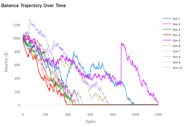
We can learn from that figure that, across the 10 simulated games, the balance tends to reach zero around 400 spins. However, some lucky runs, such as Sim 1, are able to temporarily recover losses through short winning streaks.
We can also observe the effect of the jackpot mechanism (Sim 5), which shifts a losing trajectory into a temporarily winning position, reinforcing the perception that a few players can win significantly while others lose.
Nevertheless, given enough time, even Sim 5’s final balance converges back toward zero, assuming the RTP remains unchanged throughout the process.
In general, the system recorded a total of 6,419 spins and 2 jackpot events, resulting in a jackpot frequency of approximately 1 in 3,209 spins.
Only 2 simulations experienced at least one jackpot occurrence, specifically Sim 5 and Sim 7, each with a single jackpot hit at spins 874 and 319 respectively.
The final balance distribution shows a mean final balance of $ 7.02, with values ranging from a minimum of $ 2.6 to a maximum of $ 9.8. The standard deviation is $ 2.4, indicating a moderate dispersion across simulation outcomes.
From a probabilistic standpoint, the initial RTP and all derived RTP measures remain consistent at approximately 0.8663, confirming that both the theoretical and simulated RTP converge closely.
The observed RTP from the simulation is 0.8653, which is extremely close to the expected value, reinforcing the stability of the model under repeated trials.
From this, we can conclude that the system behaves consistently under stochastic conditions, with empirical outcomes closely matching theoretical expectations.
However, this also highlights the structural asymmetry of the game: over time, the house retains a persistent advantage.
Finally, does the house always win?
Yes, it does!
But how?
To understand this, we need to look at tab_opt, which searches for the optimal configuration of weights and multipliers, ensuring that the system is tuned in a way that guarantees long-term profitability for the house.
with tab_opt:
    st.subheader("Adjust game for RTP")
    target_rtp = st.number_input("Target RTP", 0.0, 2.0, 0.96, 0.01)
    min_weight = st.number_input("Min weight", 0.1, 10.0, 0.2)
    max_weight = st.number_input("Max weight", 0.1, 10.0, 6.0)
    min_multiplier = st.number_input("Min multiplier", 1.0, 50.0, 1.5)
    max_multiplier = st.number_input("Max multiplier", 1.0, 50.0, 30.0)

    if st.button("Optimize RTP Parameters"):
        with st.spinner("Optimizing parameters..."):
            w_opt, m_opt, rtp_achieved, history = optmize_RTP(
                target_rtp,
                n_symbols=len(SYMBOLS),
                weight_bounds=(min_weight, max_weight),
                multiplier_bounds=(min_multiplier, max_multiplier),
                n_restarts=20
            )

        if w_opt is not None:
            st.write("**Optimized Parameters**")
            st.write(f"**Achieved RTP:** {rtp_achieved:.4f}")
            st.write(f"**Target RTP:** {target_rtp:.4f}")
            st.write(f"**Error:** {abs(rtp_achieved - target_rtp):.4f}")

            results_df = pd.DataFrame({
                'Symbol': SYMBOLS,
                'Weight': [f'{x:.2f}' for x in w_opt],
                'Multiplier': [f'{x:.2f}' for x in m_opt]
            })
            st.dataframe(results_df, hide_index=True)

            st.session_state.weights = w_opt
            st.session_state.multipliers = dict(zip(SYMBOLS, m_opt))

            if history:
                df_hist = pd.DataFrame({
                    "attempt": range(1, len(history) + 1),
                    "rtp": [h["rtp"] for h in history]
                })

                best_idx = (df_hist["rtp"] - target_rtp).abs().idxmin()

                fig = px.line(
                    df_hist,
                    x="attempt",
                    y="rtp",
                    markers=True
                )

                fig.add_scatter(
                    x=[df_hist.loc[best_idx, "attempt"]],
                    y=[df_hist.loc[best_idx, "rtp"]],
                    mode="markers",
                    marker=dict(size=14, color="gold", line=dict(width=2, color="black")),
                    name=f'Best: {df_hist.loc[best_idx, "rtp"]:.3f}'
                )

                fig.add_hline(
                    y=target_rtp,
                    line_dash="dash",
                    annotation_text=f"Target: {target_rtp:.3f}"
                )

                fig.add_hrect(
                    y0=target_rtp * 0.99,
                    y1=target_rtp * 1.01,
                    opacity=0.2
                )

                fig.update_layout(
                    title="RTP Optimization Progress",
                    xaxis_title="Optimization Attempt",
                    yaxis_title="RTP"
                )

                st.plotly_chart(fig, use_container_width=True)
    else:
        st.error("Optimization failed. Try adjusting bounds.")
If a slot game operates legally under national regulations, the RTP must be transparent and clearly presented to players, since it is, after all, a game of chance.
However, many online platforms operate outside proper regulation, where the house can adjust the RTP dynamically. This can be used to offer higher returns at the beginning and, as the player becomes more engaged, shift the system toward a lower RTP by making high-paying symbols rarer or reducing multipliers.
This section, tab_opt, is responsible for actively tuning the game configuration in order to match a target RTP.
The user defines a desired target_rtp, along with constraints for weights and multipliers through min_weight, max_weight, min_multiplier, and max_multiplier. These bounds control the search space in which the optimization algorithm operates.
Once triggered, the system calls optmize_RTP, which attempts multiple configurations (n_restarts) to find a combination of weights and multipliers that produces an RTP as close as possible to the target. The result includes the optimized parameters (w_opt, m_opt), the achieved rtp_achieved, and a history of attempts.
If a valid solution is found, the system reports the achieved RTP, compares it to the target_rtp, and displays the absolute error. It also presents a structured view of each Symbol alongside its corresponding Weight and Multiplier.
The optimized parameters are then persisted into st.session_state.weights and st.session_state.multipliers, meaning all subsequent simulations and game executions will use this updated configuration.
Additionally, if optimization history is available, the process is visualized over time. Each attempt is plotted against its resulting RTP, highlighting the best approximation found. A reference line marks the target_rtp, along with a tolerance band, making it easy to assess convergence and stability.
If no valid configuration is found within the defined bounds, the system returns an error, indicating that the search space may need adjustment.
When rendering it in streamlit, we come up with video 3, below:
Now consider, an experiment where:
- We optimize the initial parameters to achieve a positive RTP of 1.05.
- Players are then allowed to play 500 spins under this initial configuration.
- After that, the RTP is re-optimized to a decreasing return, for example 0.95.
- Players then continue for another 500 spins under the new configuration.
The outcome is shown in Figure 4 below:
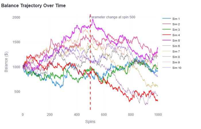
What we observe is that, among a small group of players, a significant portion initially becomes profitable, benefiting from the early positive return environment. However, after the parameter shift at 500 spins, the system starts to gradually reverse these gains.
By the end of 1000 spins, the distribution of outcomes changes drastically: some players experience full ruin, some return close to their initial balance of $1,000.00, and only a small fraction remains profitable.
Most importantly, the system naturally drifts toward a state where losses dominate over time. As the process continues, the expected equilibrium is that almost all players eventually lose their gains and return value back to the house.
Many days of struggle, a few days of glory.
Well, not for the house.
Final Thoughts
This article covered the basic concepts of gambling games, explaining how over time the player tends to lose more money than they win.
It aimed to contextualize the emotions and passions of players, who in moments of euphoria and wins tend to believe that the machine is fair and that luck favors the brave and the bold.
However, in the long run, uncertainty is structured in a way that returns less than what is wagered, and the player eventually reaches ruin.
This context raises the debate about whether casino games should be allowed in the society we live in.
Emotionally, they are forms of entertainment that separate winners from losers, the fortunate from those who were never aligned with luck.
Mathematically, they are defined toward ruin.
Sociologically, they are designed for repetition, loss cycles, and the gradual reshaping of individual behavior.
Economically, they act as a transfer of wealth from many to few, where the structural advantage always remains on the house side.
Politically, they become mechanisms for the perpetuation of financial power and the systems that sustain it.
References
WORLD HEALTH ORGANIZATION (WHO). Gambling. Geneva: WHO, 2024. Available at: https://www.who.int/news-room/fact-sheets/detail/gambling. Accessed on: 26 Mar. 2026.
TECHOPEDIA. Gambling Addiction Statistics 2024. Available at: https://www.techopedia.com/gambling-addiction-statistics. Accessed on: 26 Mar. 2026.
GROCHOWSKI, John. Double the Luck. SCCG Management, New York, 2025. Available at: https://sccgmanagement.com.
PLAYTECH. Gold Trio Jackpot & Gold Trio 10,000 — Technical Specifications. Gaming Intelligence, London, 2025. Available at: https://www.gamingintelligence.com.
SMZONE.COM.AU. The Science of Winning: Insights into Online Slot Machine Performance. smzone.com.au, Randwick, 2025. Available at: https://smzone.com.au.
MICROGAMING. Game Provider RTP and Volatility Data. In: Top 5 Game Providers Behind Goldwin Casino’s Exciting Selection. bdvo.org, 2026. Available at: https://archive2021.bdvo.org.
NETENT. Game Provider Technical Documentation. In: Top 5 Game Providers Behind Goldwin Casino’s Exciting Selection. bdvo.org, 2026. Available at: https://archive2021.bdvo.org.
ECOGRA. Testing Standards and RNG Certification. In: eebguide.eu. All Slots New Game Genres To Try This Year, 2026. Available at: https://eebguide.eu.
To bet or not to bet, that is a math question. was originally published in Level Up Coding on Medium, where people are continuing the conversation by highlighting and responding to this story.
This content originally appeared on Level Up Coding - Medium and was authored by Guilherme Ziegler

Guilherme Ziegler | Sciencx (2026-06-15T03:50:32+00:00) To bet or not to bet, that is a math question.. Retrieved from https://www.scien.cx/2026/06/15/to-bet-or-not-to-bet-that-is-a-math-question/
Please log in to upload a file.
There are no updates yet.
Click the Upload button above to add an update.