
This content originally appeared on Level Up Coding - Medium and was authored by Dinh Phu
I write practical, deep-dive articles on Data Engineering at https://dinhphuvn.substack.com/.
If you found this post helpful, you’ll definitely enjoy what’s waiting for you there. Come join a humble dev’s journey of learning, sharing, and finding joy in the process!
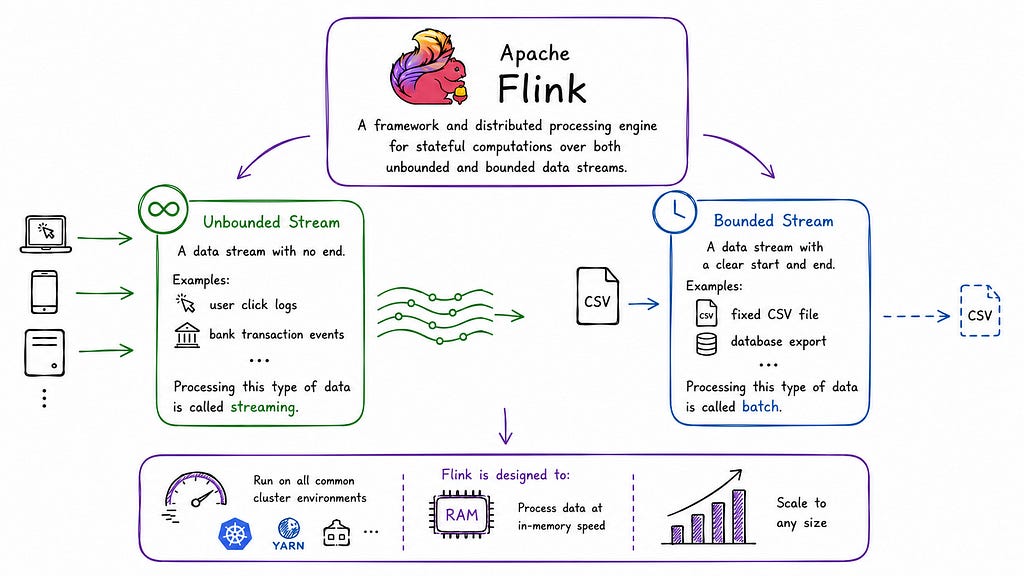
Apache Flink is a framework and a distributed processing engine used for stateful computations over both unbounded and bounded data streams.
Two key terms to remember right from the start:
- Unbounded stream: A data stream with no end — for example, user click logs or bank transaction events. Processing this type of data is called streaming.
- Bounded stream: A data stream with a clear start and end — for example, a fixed CSV file. Processing this is called batch.
Flink is designed to run on all common cluster environments, process data at in-memory speed, and scale to any size.
Flink Architecture
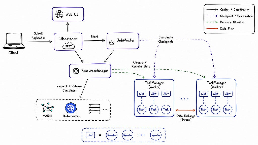
Flink’s runtime consists of two main types of processes:
JobManager
The “master” process. It coordinates the distributed execution of a Flink Application. In reality, a JobManager process includes 3 sub-components that work together:
- ResourceManager: Manages, allocates, and reclaims resources (task slots from TaskManagers). It knows how to “talk” to underlying resource managers (like YARN or Kubernetes) to request or release containers.
- Dispatcher: Provides a REST interface to accept Flink applications submitted by clients. When it receives an application, it starts the Flink WebUI and spins up a new JobMaster to manage that application.
- JobMaster: Directly manages the execution of a specific job (JobGraph). It handles the run/stop/recovery lifecycle and coordinates checkpoints. If an application has multiple jobs, each job will have its own JobMaster.
Note: In a High-Availability (HA) setup, you can run multiple JobManager processes — there is always one leader and multiple standbys, using a leader election mechanism.
TaskManager
- Also known as the “worker”. It executes the actual tasks of the dataflow, buffers data, and exchanges data between streams.
- There is always at least one TaskManager in a cluster.
- Each TaskManager is a separate JVM process.
- The smallest unit of resource scheduling in a TaskManager is a task slot. The number of slots determines how many tasks can run in parallel on that TaskManager. Note: multiple operators can share the same slot.
DataStream API and Table API/SQL
Since Flink 2.0, the DataSet API (the old API dedicated to batch) has been completely removed. If you see older documents mentioning the DataSet API, know that today Flink recommends using the DataStream API or Table API/SQL for both streaming and batch tasks.
DataStream API
This is a lower-level programming API that allows you to work directly with transformations on distributed data streams: filter, map, update state, join, group, define windows, aggregate, etc.
Data streams are created from sources (reading files, Kafka topics, or in-memory collections) and results are pushed out through sinks (writing to distributed files, or printing to the terminal).
Table API & SQL
This is a higher-level abstraction — a query API integrated into programming languages (Java, Scala, Python) that lets you build queries using relational operations (selection, filter, join) intuitively. Flink’s SQL support is powered by Apache Calcite, implementing standard SQL.
Important: Whether you write in Table API or SQL, the semantics and results are the same, regardless of whether the input is streaming or batch. These two APIs integrate seamlessly with each other and with the DataStream API — you can convert between them freely.
Core Concept of Table API/SQL: Dynamic Table
This is a concept that often confuses beginners in SQL streaming, so it needs careful understanding:
- Traditional SQL was designed for static data. But Flink SQL continuously receives new data and continuously updates the results — this is called a continuous query.
- A continuous query never ends, and always produces a dynamic table — a table whose content changes over time, similar to a materialized view in traditional databases.
- A dynamic table can be continuously modified by INSERT, UPDATE, and DELETE operations — just like a normal database table.
- When converting a dynamic table back into a stream (or writing to an external system), Flink encodes changes (Changelog) into 3 main stream types:
- Append-only stream: Only supports insert operations (INSERT).
- Retract stream: Supports INSERT, UPDATE, and DELETE. It uses “add messages” to insert and “retract messages” to remove old values. An UPDATE is encoded as a retract message for the old row followed by an add message for the new row.
- Upsert stream: Fully supports INSERT, UPDATE, and DELETE but is more efficient than Retract stream. It sends a single “upsert message” to update/insert and a “delete message” to remove. Requires the table to define a unique key (Primary Key).
Classic example: counting the number of employees per department from a continuous data stream
SELECT dept_id, COUNT(*) AS emp_count
FROM employee_information
GROUP BY dept_id;
This query is considered stateful because Flink must maintain and constantly update the latest count for each department whenever a new row of data arrives.
Event Time, Processing Time, and Watermarks
Flink supports multiple concepts of time. To see the difference, let’s use a consistent example: counting API gateway requests per minute.
Processing time
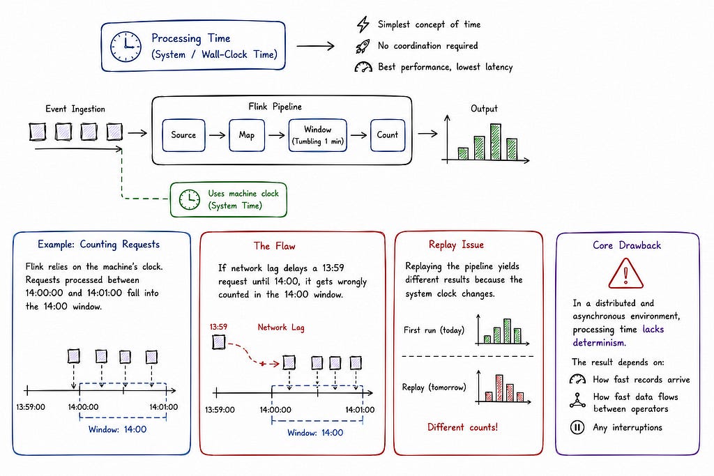
This is the system time (wall-clock time) of the machine executing the operation. It is the simplest concept of time, requiring no coordination between streams and machines, providing the best performance and lowest latency.
For example, when counting requests:
- Flink relies on the machine’s clock. Requests processed between 14:00:00 and 14:01:00 fall into the 14:00 window.
- The flaw: If network lag delays a 13:59 request until 14:00, it gets wrongly counted in the 14:00 window.
- Replay issue: Replaying the pipeline yields different results because the system clock changes.
This is the core drawback: in a distributed and asynchronous environment, processing time lacks determinism — the result depends on how fast records arrive, how fast data flows between operators, and any interruptions.
Event time
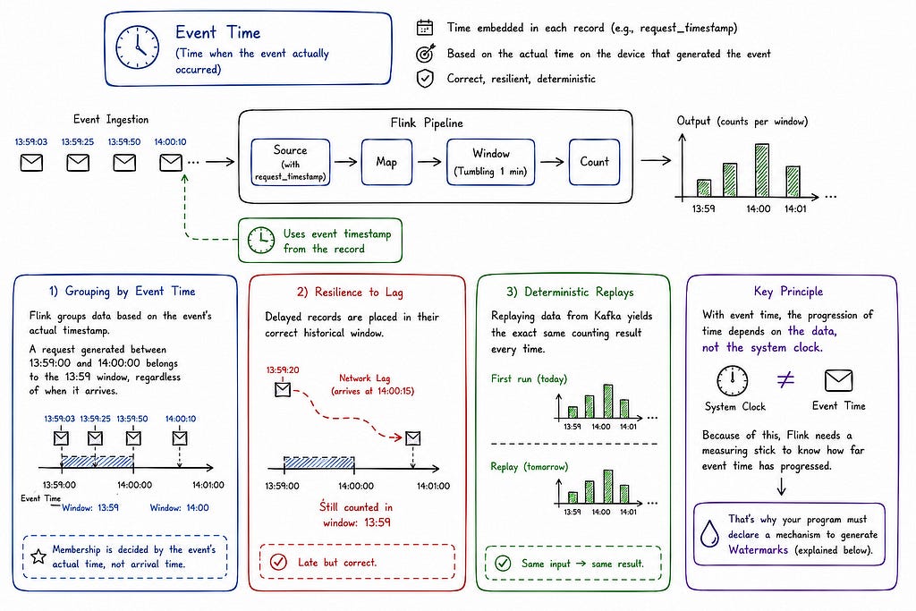
This is the time when the event actually occurred on the device that generated it, usually embedded in the record before it enters Flink.
Using the same example, but with a request_timestamp field provided by the client:
- Flink groups data based on the event’s actual timestamp. A request generated between 13:59:00 and 14:00:00 belongs to the 13:59 window, regardless of when it arrives.
- Resilience to lag: Delayed records are placed in their correct historical window.
- Deterministic replays: Replaying data from Kafka yields the exact same counting result every time.
Key principle: with event time, the progression of time depends on the data, not the system clock. But because of this, Flink needs a measuring stick to know how far event time has progressed — that is why your program must declare a mechanism to generate Watermarks (explained below).
Ingestion time (Removed in newer Flink versions)
This is the time when the event enters Flink (assigned at the source operator). Conceptually, it sits between event time and processing time: a bit more expensive than processing time but yields more predictable results; compared to event time, it cannot handle out-of-order or late data, but you don’t have to define a watermark strategy.
Important Note: The concept of Ingestion Time was deprecated in Flink 1.12 and completely removed from the documentation of newer Flink versions (like Flink 2.x). Today, you should not use Ingestion Time. Instead, use Event Time (with Watermarks assigned right at the Source) to simulate similar behavior but with more flexibility.
What is a Watermark?
Let’s continue the minute-by-minute request counting example using event time. Flink is currently opening the 13:59 window (from 13:59:00 to 14:00:00). Requests arrive one by one:
- Request X with request_timestamp = 13:59:15 → goes into the 13:59 window.
- Request Y with request_timestamp = 13:59:48 → goes into the 13:59 window.
- Request Z with request_timestamp = 14:00:03 → belongs to the 14:00 window (a new window).
The Challenge: When does Flink dare to close the 13:59 window and output the result? It cannot use the machine clock, nor can it wait forever. This is where Watermarks come into play.
How Watermarks work:
- A Watermark is a signal flowing with the data stream, carrying a timestamp t.
- It acts as a promise: no more events with a timestamp ≤ t will appear.
- Example: When Flink receives Watermark(14:00:05), it knows all 13:59 events have arrived → it safely closes the window, sums the data, and outputs the result.
Handling Late Data: What if Request W (request_timestamp = 13:59:30) arrives after the window closes due to a lagging network? This is Late Data. Flink handles it via:
- Allowed Lateness: Gives extra waiting time to update already-closed results.
- Side Output: Collects late data into a secondary stream for separate processing.
Windows: Cutting an infinite stream into finite blocks
Because a streaming flow is infinite, we cannot “sum the entire stream” — we need a way to group data into finite blocks. That is the job of a window.
A WindowAssigner is responsible for assigning each incoming element to one or more windows. Flink provides ready-to-use assigners for the most common use cases:
- Tumbling window: Windows have a fixed size and do not overlap. Each element belongs to exactly one window (unless dropped for being too late). Example: a 5-minute window, no repeating.
- Sliding window: Fixed size like tumbling, but windows can overlap. The overlap is determined by the “window slide” parameter. Example: a 10-minute window, sliding every 5 minutes — meaning every 5 minutes you get a result calculated over the last 10 minutes of data. Because of overlapping, an element can belong to multiple windows at once.
- Session window: Suitable when the window boundaries need to adjust based on the incoming data itself. Unlike tumbling and sliding (which have fixed start points and fixed sizes), a session window has a per-key start point, and it closes when there is a certain period of inactivity (a gap).
- Global window: Groups all elements with the same key into a single window — usually requires a custom trigger because it never closes on its own.
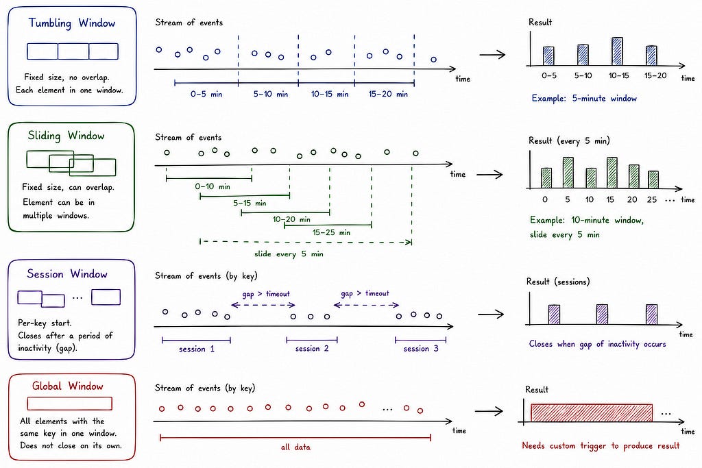
All built-in window assigners (except global window) group elements based on time — which can be processing time or event time, depending on your configuration.
State: The core mechanism of “stateful stream processing”
The phrase “stateful computations” in Flink’s definition is no accident. Consider a simple problem: counting the number of requests each user sends to an API gateway. Every time a new request arrives, Flink must know how many requests that user has sent previously to add 1. The number of “previous requests” is the state — the thing Flink must remember between records.
Without state, each record comes and goes, and Flink remembers nothing — like a computer without a hard drive. With state, Flink becomes an engine with memory, capable of accumulating and computing continuously on an infinite data stream.
Besides counting, state is also needed when:
- Searching for event sequences by pattern — state saves the sequence matched so far.
- Aggregating data over time windows — state holds the pending aggregated value.
- Training ML models on a data stream — state holds current model parameters.
For state to be fault-tolerant, Flink needs to be aware of that state and periodically checkpoint it.
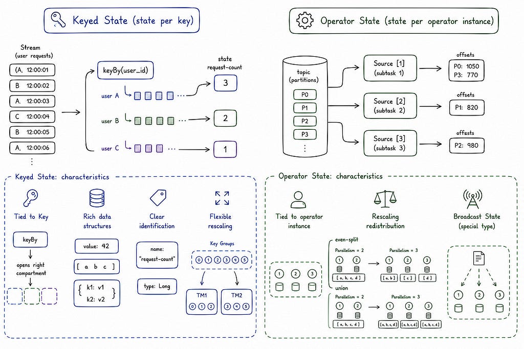
Keyed State — state per key
Back to the user request counting example. After calling keyBy(user_id), Flink splits the data stream by user: all requests from user A go into one “compartment”, all requests from user B go into another. Each compartment keeps its own separate counter (state) — this is Keyed State.
Characteristics:
- Automatically tied to the Key: Can only be used after you partition the stream using keyBy. When processing user A’s data, Flink automatically “opens the right compartment” containing user A’s state for you.
- Rich data structures: Depending on your needs, you can store state as a single value (a counter), a list (access history), or a map (key-value dictionary).
- Clear identification: For Flink to manage it, you just need to give the state a name (e.g., “request-count”) and tell Flink what data type you want to store. Flink takes care of all the complex underlying storage.
- Flexible Rescaling: If you add servers to process faster, Flink groups these states into small clusters called Key Groups and automatically moves them to new machines without losing or corrupting data.
Operator State — state per operator instance
Not all state is tied to a specific key. Consider a Kafka source connector: each parallel instance of the source reads a specific set of partitions and needs to remember its current offset. This offset is not related to any key in the data — it is tied to the operator instance itself. This is Operator State.
Characteristics:
- Each state is tied to a specific parallel instance of the operator, independent of keys.
- When changing parallelism (rescaling), Flink redistributes Operator State using these mechanisms: even-split (distributing the list of states evenly among new instances) or union (each new instance receives the entire state).
- Broadcast State is a special type of Operator State — used when all subtasks need to keep identical copies of the state. For example: a stream containing a set of rules that must be sent to all subtasks to evaluate against the main data stream.
State Backend: Where State is Stored
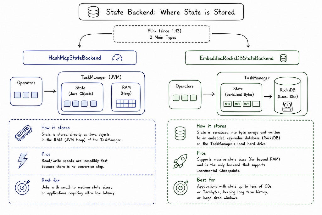
The decision of where to store state and how is managed by Flink through a component called the State Backend. Since Flink 1.13, this architecture is standardized into 2 main types:
- HashMapStateBackend:
- How it stores: State is stored directly as Java objects in the RAM (JVM Heap) of the TaskManager.
- Pros: Read/write speeds are incredibly fast because there is no conversion step (serialize/deserialize).
- Best for: Jobs with small to medium state sizes, or applications requiring ultra-low latency.
2. EmbeddedRocksDBStateBackend:
- How it stores: State is serialized into byte arrays and written to an embedded key-value database called RocksDB (stored on the TaskManager’s local hard drive).
- Pros: Supports massive state sizes (far exceeding the machine’s RAM capacity) and is the only backend that supports Incremental Checkpoints (only backing up newly changed data).
- Best for: Applications with state up to tens of GBs or Terabytes, keeping long-term history, or running large-sized windows.
Fault tolerance: Checkpoints and Savepoints
This area best demonstrates Flink’s “exactly-once” philosophy — and is also the most frequently misunderstood topic.
How does the checkpoint mechanism work?
Flink uses a variation of the Chandy-Lamport algorithm, called asynchronous barrier snapshotting. Imagine data as a continuously flowing river, and Flink drops “marker lines” (called Stream Barriers) into that river. These barriers divide the infinite data stream into finite chunks.
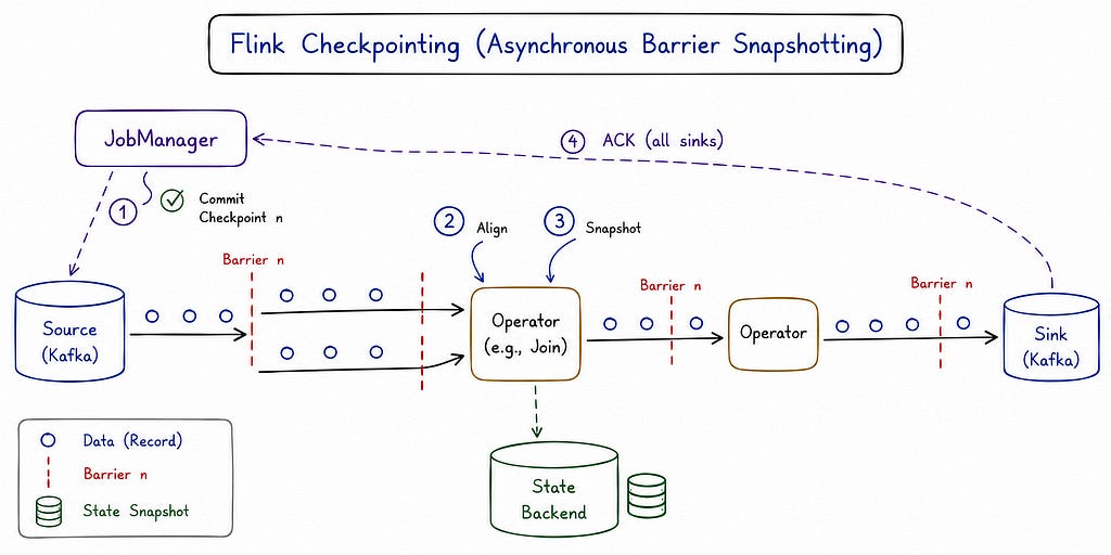
The process unfolds in 4 intuitive steps:
- Drop Barrier from Source: The JobManager (the coordinator) commands the Sources (e.g., Kafka) to drop a Barrier numbered n into the data stream. This Barrier flows downstream alongside the actual data (records).
- Alignment: When Barrier n reaches an intermediate operator, this operator does something crucial: It waits. If it receives data from multiple streams (like in a join operation), it temporarily stops processing the stream that already received the Barrier, and waits until it receives Barrier n from all remaining input streams.
- Snapshot the State: The exact moment it receives Barrier n from every input stream, the operator is 100% certain that: “I have completely processed all data before Barrier n, and I haven’t touched any data after Barrier n yet”. Immediately, it captures its entire current State and backs it up to the State Backend.
- Propagate and Commit: After taking the snapshot, it pushes Barrier n further downstream to the next operators. The process continues until the Barrier reaches the Sinks (the final data output points). When all Sinks acknowledge completion, the JobManager “commits” that Checkpoint n is successfully done!
Aligned vs. Unaligned Checkpoints
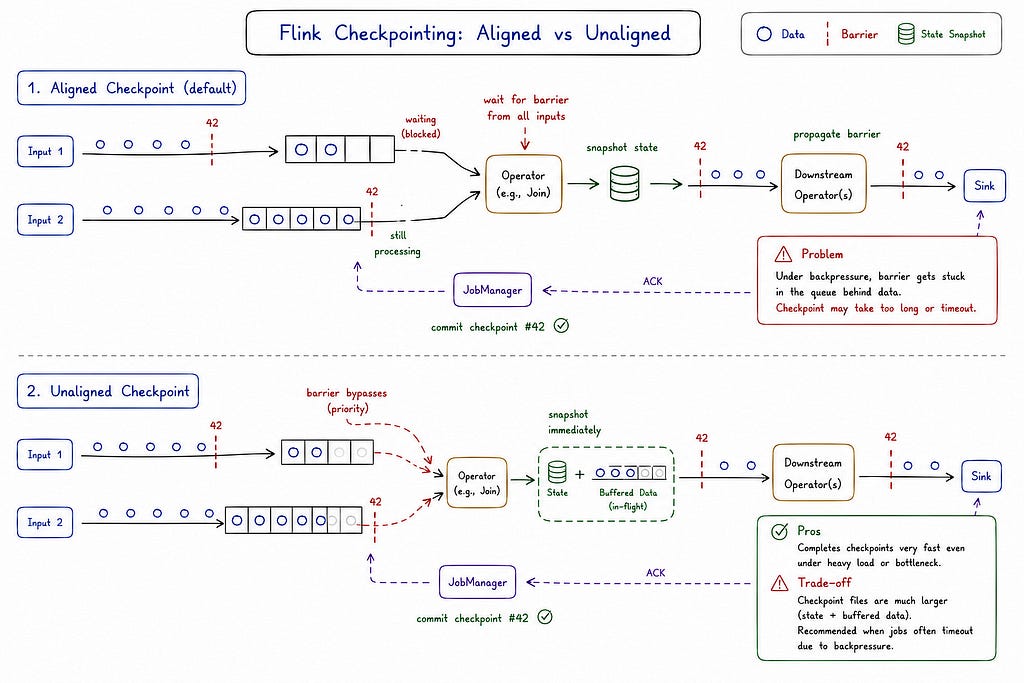
The “wait and commit” mechanism in Step 2 is called an Aligned Checkpoint. Its fatal flaw is that when the system is congested (backpressure), the Barrier gets stuck in the queue along with data, causing the Checkpoint to take too long or timeout.
To rescue the situation, Flink provides Unaligned Checkpoints. In this mode, the Barrier is granted priority to bypass all stuck data to trigger the State snapshot immediately. To guarantee no data discrepancy, Flink is forced to save both the operator’s State and all the data stuck in the queue into the Checkpoint file.
- Pros: Completes Checkpoints extremely fast even under heavy load or bottlenecks.
- Trade-off: The Checkpoint file size is much larger. Recommended when your job constantly faces Checkpoint timeouts due to backpressure.
What is the difference between a Checkpoint and a Savepoint?
This is almost a “must-have” interview question when discussing Flink. The official documentation makes an analogy: the difference between a checkpoint and a savepoint is like the difference between a backup and a recovery log in a traditional database management system.
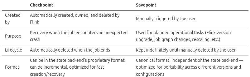
In short: checkpoints are for automatic crash recovery, savepoints are for you to proactively “package” the job state for maintenance, upgrades, or moving jobs.
Deployment Modes
How you deploy Flink determines two core factors: cluster lifecycle (how long it exists) and where the main() method is executed (on your machine or on the server).
From Flink 2.x, the deployment architecture is streamlined into just two main modes:
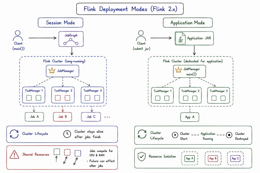
Session Mode: Shared Resources
- Mechanism: You start a cluster in advance. Then you submit multiple jobs consecutively to this cluster.
- main() Execution: Runs on the Client machine. The Client machine loads the code, translates it into a JobGraph, and only then pushes it over the network to the cluster.
- When to use: When you have many small, fast-running jobs and don’t want to incur the overhead of creating a new cluster every time.
- Weakness: “Domino effect” risk. Jobs will compete for CPU and RAM. If one job crashes and takes down a TaskManager, all other jobs running on that TaskManager will crash too.
Application Mode: Resource Isolation
- Mechanism: Flink creates a brand new cluster exclusively to serve your application. When the application finishes, the cluster is automatically destroyed.
- main() Execution: Runs directly on the JobManager. The .jar file containing your code is packaged straight into the Flink image instead of being sent from the Client.
- When to use: For Production environments because applications are completely independent and won’t spread errors to each other.
- Weakness: Takes extra time to initialize the cluster at the beginning.
Conclusion
This article has gotten quite long, and we’ve really only scratched the surface of Flink’s core concepts. I will be writing more in-depth, deep-dive articles for each of these specific topics in the future, so stay tuned!
Hopefully, this guide has demystified Flink’s core architecture and equipped you with the mental models needed for your upcoming production projects. Happy streaming!
References
Apache Flink from A to Z: The Engineer’s Guide to Stream Processing was originally published in Level Up Coding on Medium, where people are continuing the conversation by highlighting and responding to this story.
This content originally appeared on Level Up Coding - Medium and was authored by Dinh Phu

Dinh Phu | Sciencx (2026-07-24T14:12:48+00:00) Apache Flink from A to Z: The Engineer’s Guide to Stream Processing. Retrieved from https://www.scien.cx/2026/07/24/apache-flink-from-a-to-z-the-engineers-guide-to-stream-processing/
Please log in to upload a file.
There are no updates yet.
Click the Upload button above to add an update.